In the previous post we saw how to fit simple GAM using the mgcv package. We also saw how to plot and check a fitted gam and discussed some of the details behind the plots and checks. This time we will see how we can extend our model to incorporate more terms and how we can combine those terms in different ways to get different types of models. My hope is that this demonstrates the flexibility of GAMs that I mentioned previously. We won’t be building up to a single, final model as one would do if they were doing a real analysis. Rather, we will see what types of terms GAMs can handle and the different ways in which they can be combined.
The Data
We will be using the Ames Housing Dataset as before. But this time we will be including two more variables. Last time we modeled the sale price of a home as a smooth function of the lot size. This time we will add in the above ground square footage and the building type. There are a lot of other variables in this data set but to keep things manageable we will only be looking at these three. We saw before that both sale price and lot area warranted log transformations. We will stick with these transformations and also log transform the square footage of the house.
library(tidyverse)
library(mgcv)
library(AmesHousing)


ames <- make_ames() %>%
  select(Sale_Price,
         Lot_Area,
         Bldg_Type,
         Gr_Liv_Area)

names(ames) <- tolower(names(ames))

ames <- ames %>%
  mutate(log_sale_price = log(sale_price),
         log_lot_area = log(lot_area),
         log_sf = log(gr_liv_area))
As a reminder, this is what the model from last time looked like.
log_log_lot_area <- gam(log_sale_price ~ s(log_lot_area),
                    data = ames,
                    method = "REML")

summary(log_log_lot_area)
##
## Family: gaussian
## Link function: identity
##
## Formula:
## log_sale_price ~ s(log_lot_area)
##
## Parametric coefficients:
## Estimate Std. Error t value Pr(>|t|)
## (Intercept) 12.020969 0.006693 1796 <2e-16 ***
## ---
## Signif. codes: 0 '***' 0.001 '**' 0.01 '*' 0.05 '.' 0.1 ' ' 1
##
## Approximate significance of smooth terms:
## edf Ref.df F p-value
## s(log_lot_area) 8.449 8.914 86.9 <2e-16 ***
## ---
## Signif. codes: 0 '***' 0.001 '**' 0.01 '*' 0.05 '.' 0.1 ' ' 1
##
## R-sq.(adj) = 0.21 Deviance explained = 21.2%
## -REML = 1205 Scale est. = 0.13125 n = 2930One Smooth, One Factor
For the first extension of our previous model we will include the building type, a factor, in addition to the smooth for lot area.
area_type <- gam(log_sale_price ~ s(log_lot_area) + bldg_type,
                 data = ames,
                 method = "REML")

summary(area_type)
##
## Family: gaussian
## Link function: identity
##
## Formula:
## log_sale_price ~ s(log_lot_area) + bldg_type
##
## Parametric coefficients:
## Estimate Std. Error t value Pr(>|t|)
## (Intercept) 11.972870 0.007734 1548.057 < 2e-16 ***
## bldg_typeTwoFmCon -0.271036 0.044462 -6.096 1.23e-09 ***
## bldg_typeDuplex -0.171485 0.033815 -5.071 4.20e-07 ***
## bldg_typeTwnhs 0.559194 0.060078 9.308 < 2e-16 ***
## bldg_typeTwnhsE 0.514793 0.032910 15.642 < 2e-16 ***
## ---
## Signif. codes: 0 '***' 0.001 '**' 0.01 '*' 0.05 '.' 0.1 ' ' 1
##
## Approximate significance of smooth terms:
## edf Ref.df F p-value
## s(log_lot_area) 8.148 8.805 115.3 <2e-16 ***
## ---
## Signif. codes: 0 '***' 0.001 '**' 0.01 '*' 0.05 '.' 0.1 ' ' 1
##
## R-sq.(adj) = 0.288 Deviance explained = 29.1%
## -REML = 1058.7 Scale est. = 0.11835 n = 2930Since building type is a factor and we included it as a linear term, gam considers it a parametric term. This means that building type is included as a dummy variable just like in an lm model. But note that the smooth term is different from when we didn’t include building type. If we pass this model to plot we will again get a plot of the smooth term.
One Smooth Per Level
What if we wanted to include a separate smooth term for each level of building type? This might make more sense because the lot area of say a townhouse will likely be different than the lot area of a single family home. To do this, we need to put building type inside the smoother s().
area_by_type <- gam(log_sale_price ~ s(log_lot_area, by = bldg_type),
                    data = ames,
                    method = "REML")
summary(area_by_type)
##
## Family: gaussian
## Link function: identity
##
## Formula:
## log_sale_price ~ s(log_lot_area, by = bldg_type)
##
## Parametric coefficients:
## Estimate Std. Error t value Pr(>|t|)
## (Intercept) 11.98379 0.01531 783 <2e-16 ***
## ---
## Signif. codes: 0 '***' 0.001 '**' 0.01 '*' 0.05 '.' 0.1 ' ' 1
##
## Approximate significance of smooth terms:
## edf Ref.df F p-value
## s(log_lot_area):bldg_typeOneFam 7.443 8.092 114.481 < 2e-16 ***
## s(log_lot_area):bldg_typeTwoFmCon 6.294 7.193 5.245 4.97e-06 ***
## s(log_lot_area):bldg_typeDuplex 2.735 3.347 3.308 0.0161 *
## s(log_lot_area):bldg_typeTwnhs 2.676 3.040 27.842 < 2e-16 ***
## s(log_lot_area):bldg_typeTwnhsE 5.395 6.064 16.346 < 2e-16 ***
## ---
## Signif. codes: 0 '***' 0.001 '**' 0.01 '*' 0.05 '.' 0.1 ' ' 1
##
## R-sq.(adj) = 0.289 Deviance explained = 29.5%
## -REML = 1074.7 Scale est. = 0.11804 n = 2930Now the levels of building type have shifted from the parametric terms section to the smooth terms section. For each level of building type, we have a different smooth of lot area. Let’s see what happens when we plot this model.
plot(area_by_type,
     residuals = TRUE,
     rug = FALSE,
     shade = TRUE,
     shift = coef(area_by_type)[1],
     seWithMean = TRUE,
     pages = 1)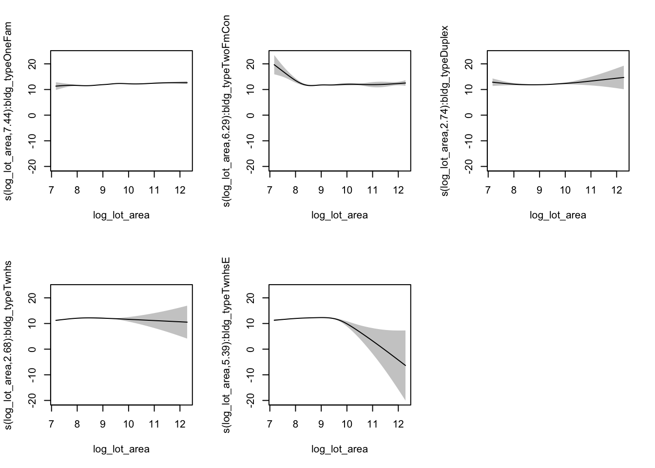
We get a plot of each one of the smooths. Note the additional argument pages = 1 to the plot. This just says we want all our plots on the same page, instead of five separate plots. Also note that we can draw a horizontal line through the confidence intervals of some of these smooths so we probably shouldn’t include building type as we did.
Two Smooths
Let’s forget about building type for now and add in the size of the house. We could include it as a linear term but let’s try it as an additional smooth term.
area_sf <- gam(log_sale_price ~ s(log_lot_area) + s(log_sf),
               data = ames,
               method = "REML")
summary(area_sf)
##
## Family: gaussian
## Link function: identity
##
## Formula:
## log_sale_price ~ s(log_lot_area) + s(log_sf)
##
## Parametric coefficients:
## Estimate Std. Error t value Pr(>|t|)
## (Intercept) 12.020969 0.004986 2411 <2e-16 ***
## ---
## Signif. codes: 0 '***' 0.001 '**' 0.01 '*' 0.05 '.' 0.1 ' ' 1
##
## Approximate significance of smooth terms:
## edf Ref.df F p-value
## s(log_lot_area) 8.535 8.938 24.44 <2e-16 ***
## s(log_sf) 7.580 8.510 275.41 <2e-16 ***
## ---
## Signif. codes: 0 '***' 0.001 '**' 0.01 '*' 0.05 '.' 0.1 ' ' 1
##
## R-sq.(adj) = 0.562 Deviance explained = 56.4%
## -REML = 357.69 Scale est. = 0.072832 n = 2930Again, we only have the intercept in the parametric section because we didn’t add any linear terms. But now we have one smooth for lot area and one smooth for the square footage of the house. What will a plot look like when we have more than one smooth term? We get two plots, one for each smooth.
plot(area_sf,
     residuals = TRUE,
     rug = FALSE,
     shade = TRUE,
     shift = coef(area_sf)[1],
     seWithMean = TRUE,
     pages = 1)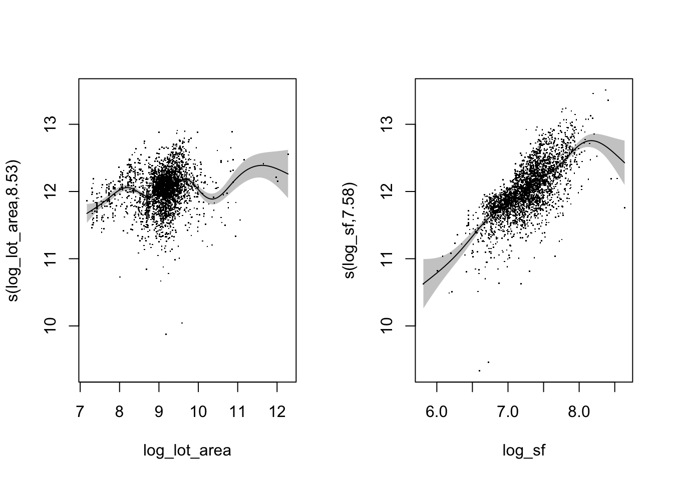
One Smooth, Two Variables
We just saw what happens when we include two separate smooth terms. But what if we wanted to include a single smooth term that takes into account two variables? This might be useful for example in a spatial problem when you have latitude and longitude. It would probably make more sense to combine them in a single smooth rather than treat them separately. We can incorporate this into a GAM by using s(x1, x2) like this:
area_sf_interact <- gam(log_sale_price ~ s(log_lot_area, log_sf),
                        data = ames,
                        method = "REML")
Passing both lot area and square footage to s() takes into account lot area, square footage, and their interaction into a single smooth term. In this case we have a two dimensional smooth so the plot of this model is going to be different than what we’ve seen so far. By default a contour plot is produced. Plots of the standard error are also given but this time at \(\pm\) 1 standard error instead of two. Other options include a perspective plot (surface plot), and two types of heatmaps. I prefer perspective plots so let’s do that here.
plot(area_sf_interact,
     scheme = 1)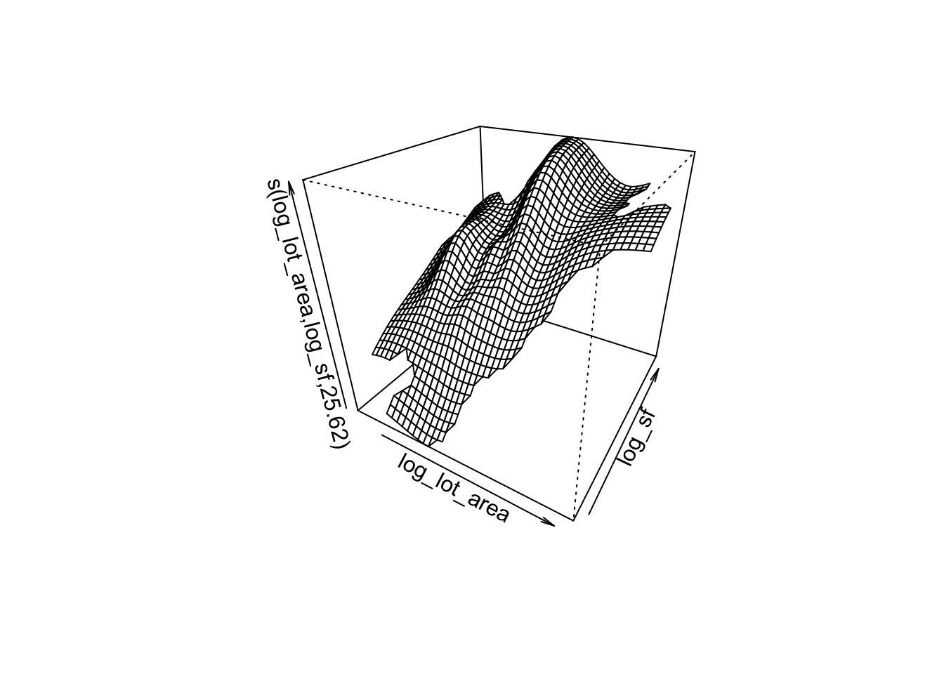
We get a plot of the smooth as a function of each of the smoothed variables, lot area and square footage. We could customize plot a bit more depending on what we want. Or we could use another function, vis.gam which is meant for 3d plots. Not only that, but instead of plotting the smooth, it plots the predictor.
vis.gam(area_sf_interact,
        view = c("log_lot_area", "log_sf"),
        plot.type = "persp",
        theta = 45)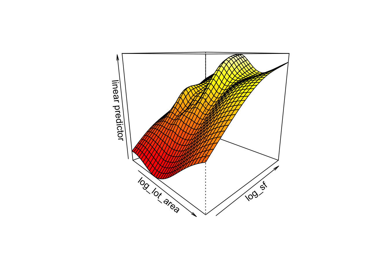
A Note
Hopefully what we did here gives you a better understanding of what we can do with GAMs and how flexible they are. I think this flexibility is great but there is a cost to it. Because we can combine different types of terms in different ways, we have a lot of options when building a GAM, possibly too many. For a problem with a handful of covariates and a lot of domain knowledge, this shouldn’t be an issue. But let’s say you have a data set with 50 variables of different types and you don’t have any knowledge of the underlying subject. In that case I don’t think a GAM would be a good option because there are just too many ways to combine that many variables. For instance, should you use a separate smooth for each numeric variable? Which numeric variables should have interactions? Which numeric variables should include a separate smooth for each level of a factor? Usually we are concerned with which variables to include but with GAMs we also need to consider how we are going to include them. Anyways, just like anything else, GAMs can be great but it really depends on the problem at hand.