Generalized Additive Models Part 2: A First GAM

The Data

For this post we will be using the Ames Housing Dataset. The Ames Housing R package provides the original data set along with a cleaned version of the data. We will be using a subset of the cleaned data set. Specifically, we will be modeling the sale price of a house as a function of the lot size. This is probably not the best single variable model but that isn’t the focus of this post. I really just want to demonstrate how to use the mgcv package.

library(tidyverse)
library(mgcv)
library(AmesHousing)

ames <- make_ames() %>% 
  select(Sale_Price,
         Lot_Area)

names(ames) <- tolower(names(ames))

Let’s look at a plot of sale price vs. lot area to get a feel for the relationship between them.

ggplot(ames, aes(lot_area, sale_price)) +
  geom_point()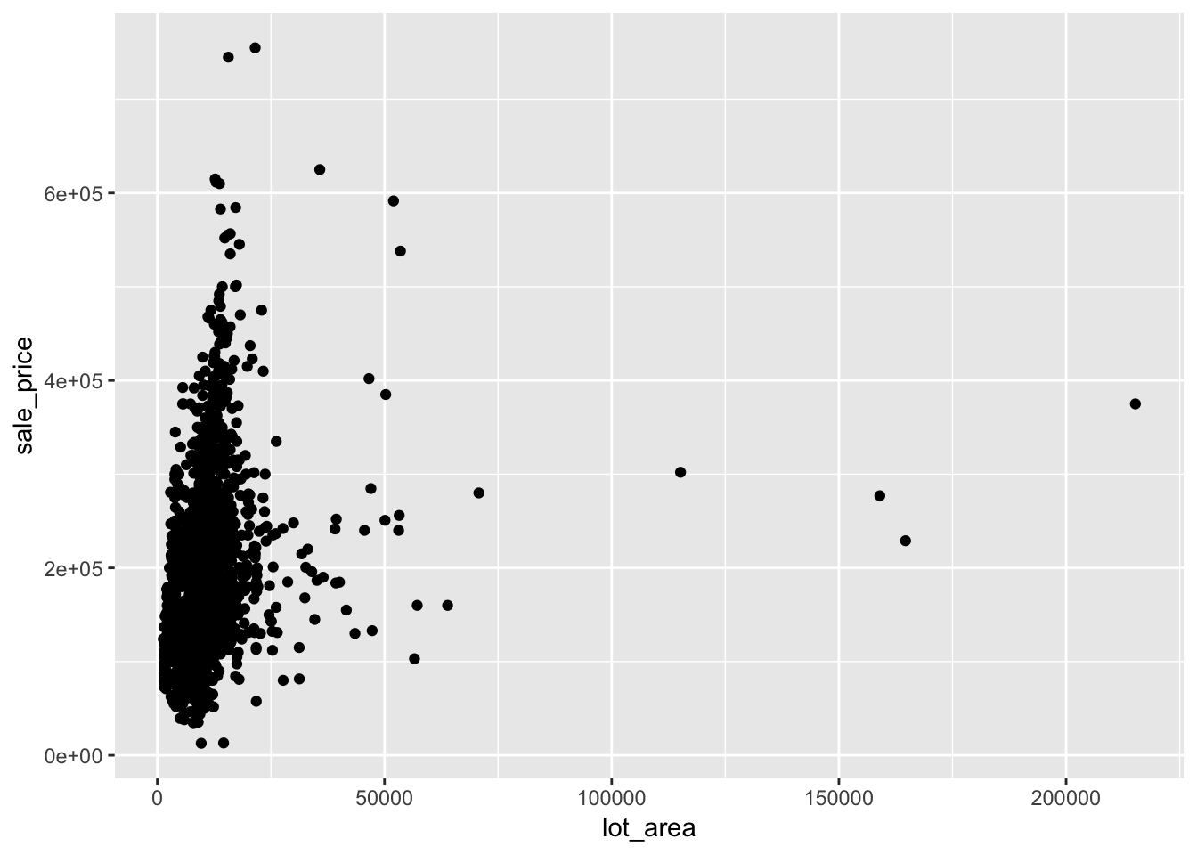

This doesn’t look so good. Besides the few extreme values, everything looks bunched up. We can see if a log transformation helps.

ggplot(ames, aes(lot_area, sale_price)) +
  geom_point() +
  scale_x_log10() +
  scale_y_log10()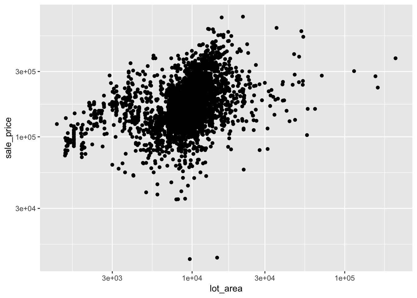

This looks better. There isn’t an obvious relationship here but it is obvious that the relationship is not linear. Good thing we are using nonlinear models. Actually, it would be fine if the relationship was linear because, as we will see shortly, mgcv has a way of telling you if there is a linear relationship.

Our First GAM

Alright, let’s go ahead and fit a GAM to see what it looks like and what we can do with it. Based on what we saw in the plots, we will use log transformed versions of sale price and lot area.

ames <- ames %>% 
  mutate(log_sale_price = log(sale_price),
         log_lot_area = log(lot_area))

log_log_lot_area <- gam(log_sale_price ~ s(log_lot_area),
                    data = ames,
                    method = "REML")

Let’s break down what is going on here. To fit a GAM in mgcv we use the function … gam. The s() function wrapped around lot area tells gam we want to use a smooth version of lot area and not lot area itself. By default it uses a thin plate spline but there are other options. For example, we could use a cubic spline basis with s(x, bs = "cr"). The method argument specifies we want to use restricted maximum likelihood. I’ve heard it’s best to use REML in most cases so that’s what we are going to stick with here.

Now let’s investigate our fit by trying a few things out. We will start with just printing the model and then look at what methods are available.

log_log_lot_area

## 
## Family: gaussian 
## Link function: identity 
## 
## Formula:
## log_sale_price ~ s(log_lot_area)
## 
## Estimated degrees of freedom:
## 8.45  total = 9.45 
## 
## REML score: 1204.978

methods(class = "gam")

##  [1] anova          cooks.distance formula        influence     
##  [5] logLik         model.matrix   plot           predict       
##  [9] print          residuals      summary        vcov          
## see '?methods' for accessing help and source code

Great, we have a summary method. What does that do?

summary(log_log_lot_area)

## 
## Family: gaussian 
## Link function: identity 
## 
## Formula:
## log_sale_price ~ s(log_lot_area)
## 
## Parametric coefficients:
##              Estimate Std. Error t value Pr(>|t|)    
## (Intercept) 12.020969   0.006693    1796   <2e-16 ***
## ---
## Signif. codes:  0 '***' 0.001 '**' 0.01 '*' 0.05 '.' 0.1 ' ' 1
## 
## Approximate significance of smooth terms:
##                   edf Ref.df    F p-value    
## s(log_lot_area) 8.449  8.914 86.9  <2e-16 ***
## ---
## Signif. codes:  0 '***' 0.001 '**' 0.01 '*' 0.05 '.' 0.1 ' ' 1
## 
## R-sq.(adj) =   0.21   Deviance explained = 21.2%
## -REML =   1205  Scale est. = 0.13125   n = 2930

There are two main sections here, ‘Parametric coefficients’ and ‘Approximate significance of smooth terms’. The parametric section gives the standard summary for the non-smooth terms; in this case we only have the intercept. The next section describes our smooth term s(log_lot_area). The first column, edf, is the effective degrees of freedom of the term, the trace of the smoother (or hat) matrix. When the degrees of freedom is 1, this is a linear term. So GAMs don’t try to force nonlinearity. If a term should be linear, gam will figure it out. If you’re unsure whether a variable should be included linearly in a model, gam can help you figure this out. Another nice thing about the degrees of freedom is 2 degrees of freedom corresponds to a quadratic, 3 to a cubic, etc. The next three columns provide information regarding a test of significance for the smooth term. The null is that the whole smooth term s(log_lot_area) is zero. The p-value here is an approximation and shouldn’t be taken too seriously.

Plotting Our GAM

Another way to assess whether a smooth term should be included is by examining a partial effects plot which we will look at now. We’ll start by using all the default arguments just to see what that looks like.

plot(log_log_lot_area)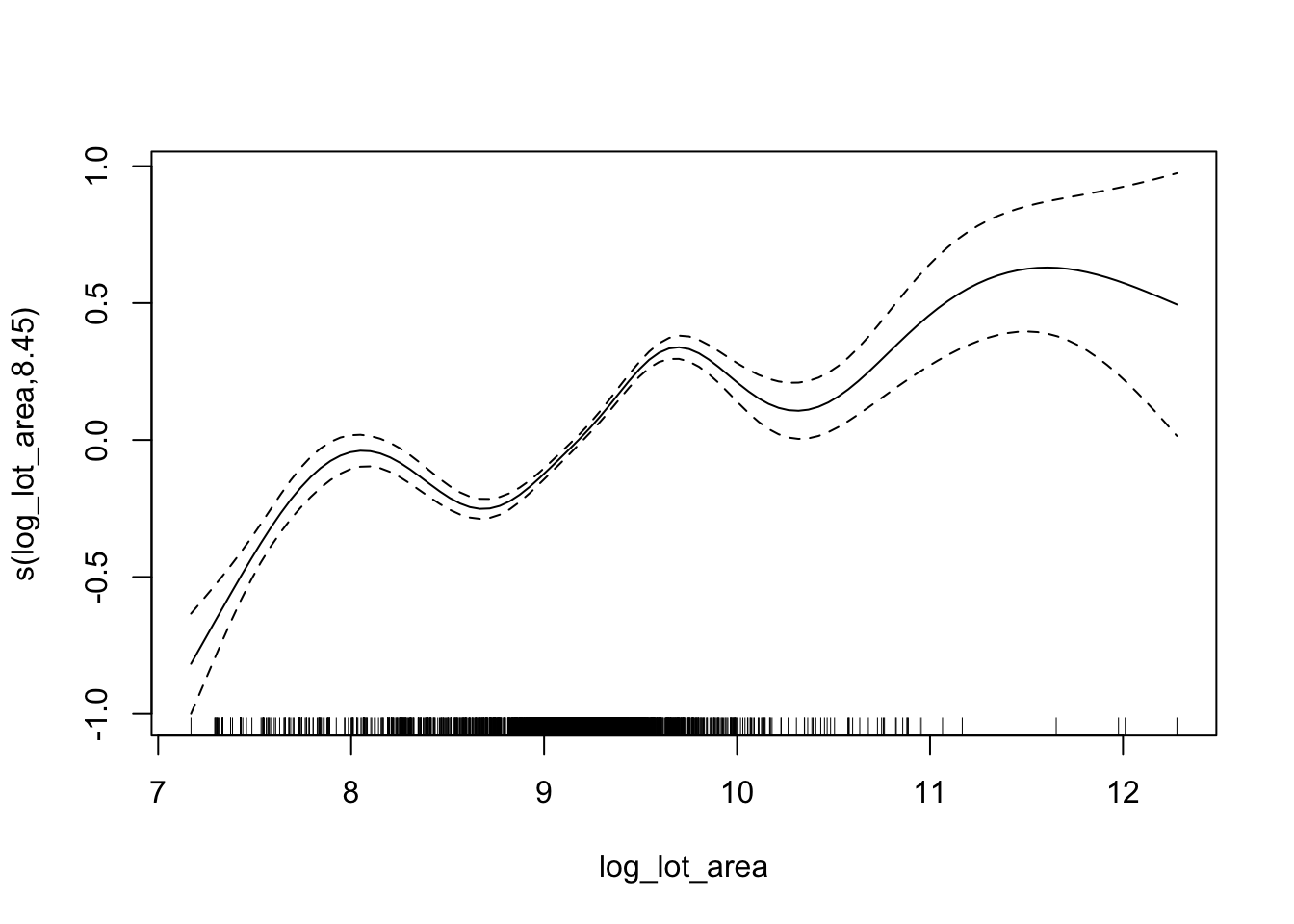

This gives us a plot of the variable of interest vs. its smooth version. Also plotted is the smooth with \(\pm\) 2 standard errors added on, essentially showing a 95% confidence interval. We can assess whether or not this term should be included using the following rule-of-thumb: if we can draw a horizontal line through the confidence interval, it should not be included. In this case we can’t do that so we would want to keep this term. Let’s change a few of the plotting arguments to get a feel for what kind of control we have.

plot(log_log_lot_area,
     residuals = TRUE,
     rug = FALSE,
     shade = TRUE,
     shift = coef(log_log_lot_area)[1],
     seWithMean = TRUE)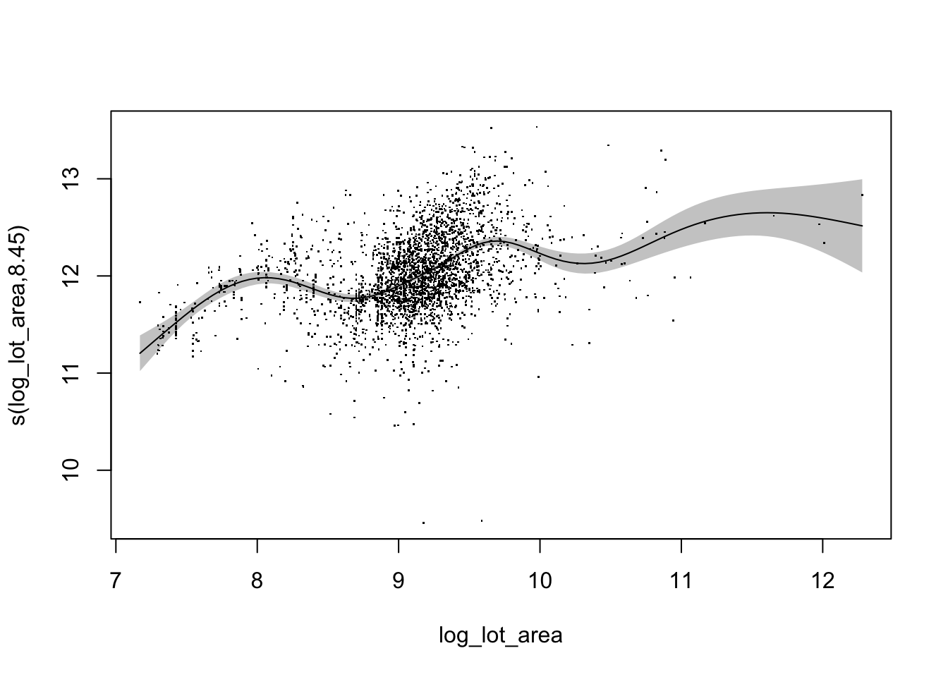

This is a bit more complex than the first call to plot so let’s describe what each one of these arguments does. We’ll start with shade because that’s the most obvious: should we shade the confidence region? Similarly, rug specifies whether or not a rug is added to the plot. I rarely use these and with the residuals added, I don’t really see a benefit to a rug as well. And that brings us to the residuals argument. These are actually partial residuals. The documentation describes them as:

Partial residuals for a smooth term are the residuals that would be obtained by dropping the term concerned from the model, while leaving all other estimates fixed.

So if we did not have s(log_lot_area) in the model, and just the intercept, the residuals would be the points shown in the graph. The shift argument just adds a constant to the smooth. In this case we are adding on the intercept. This gives us a better sense of what is going on because it shows how the smooth effects the (log) sale price. The first smooth plot ranges from -1 to 1 which doesn’t really tell us as much about the response. And finally we have seWithMean. When TRUE, the uncertainty of the mean is incorporated into the confidence band. If FALSE, only the uncertainty of the smooth is used.

Checking Our GAM

We already saw how to assess if a smooth term should be included in our model via p-values and the ‘line test’. If we are satisfied with this and want to go further with diagnosing our model we can use the gam.check function. This function provides us with diagnostic information in the form of plots and summary numbers. The plots are of the residuals and the numbers tell us about convergence and the dimension of the basis for the smooth. Let’s see what this looks like for our model:

gam.check(log_log_lot_area)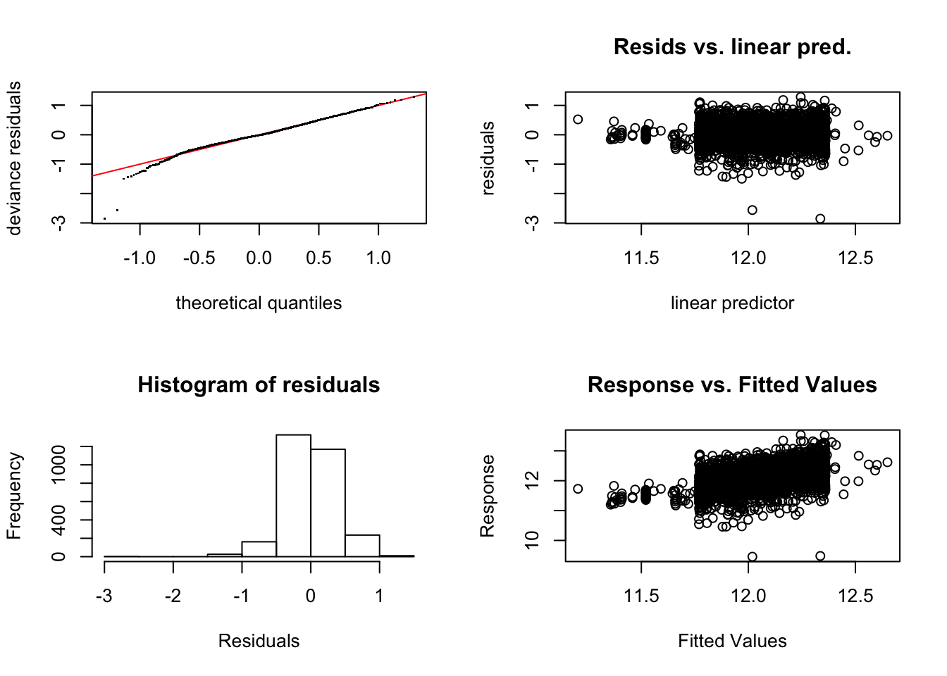

## 
## Method: REML   Optimizer: outer newton
## full convergence after 5 iterations.
## Gradient range [-0.000759463,2.576653e-05]
## (score 1204.978 & scale 0.1312532).
## Hessian positive definite, eigenvalue range [3.143352,1464.01].
## Model rank =  10 / 10 
## 
## Basis dimension (k) checking results. Low p-value (k-index<1) may
## indicate that k is too low, especially if edf is close to k'.
## 
##                   k'  edf k-index p-value    
## s(log_lot_area) 9.00 8.45    0.91  <2e-16 ***
## ---
## Signif. codes:  0 '***' 0.001 '**' 0.01 '*' 0.05 '.' 0.1 ' ' 1

As we can see, the plots generated are the usual residual diagnostic plots. As for the numeric summaries, the convergence stuff probably won’t matter in most cases. The important thing is that the model did converge. What we care about more is the second part. Basically, a test is run to see of the dimension of the basis for the smooth is too low. If it is, we are probably over smoothing and want some more wiggliness. Be careful with the p-value here as it is opposite of what we are used to. If we have a good basis dimension, the p-value will be high. If the p-value is low, it indicates problems. In our case the p-value is really small so we may need a higher dimensional basis. We can do this with something like s(log_lot_area, k = 30) but we won’t worry about it here. Also note the print out helpfully tells us that low p-values are especially troublesome when our effective degrees of freedom are close to k' which is the case in this model.

Next Steps

Hopefully by now you have a basic understanding of how you might use a GAM with the mgcv package. In the next post we will dig a little deeper by seeing how to fit different types of GAM models. We will mix different types of terms and different types of smooths in order to illustrate the flexibility GAMs.