GAMs for Time Series

Last Time

Last time we used a GAM to model the number of flu-like illnesses reported to the CDC using three different approaches. We started by using time as a predictor variable of the form \(t = 1,2,3, ...\). This did not go well. The second approach we used had smooth functions of year and week as predictors. This gave a reasonable fit to the data but the forecasts were terrible. Lastly, we used four weeks worth of lags as predictors and this gave us a good fit to the data as well as excellent forecasts.

I have to admit that going into the that post I was pretty lost as to how we could actually extend GAMs to time series. Time series models explicitly account for time and autocorrelation. However, GAMs are generic models so we need to specify how to account for this ourselves. We need to tell the model not just what are predictors are but how we want them to be handled.

This Time

In this post we are going to investigate the different ways in which we can model time series with GAMs. We will look at how we might want to use time as predictors, including functions of time in various ways by using different smoothing bases, and how to account for autocorrelation. We will stick with the flu-like illness data because it has proven itself to be a bit finicky.

Resources

Before we start I’d like to point out a few resources because if not for them I would still be lost. The first is Noam Ross’s GAM resources GitHub repository. This is just what it sounds like, a list of resources for learning about GAMs. Of particular interest to me were the slides and video for his talk outlining what GAMs and the mgcv package are capable of. One section of this talk is dedicated to time series which really got the ball rolling for me. The second resource I found really helpful is Gavin Simpson’s blog post showing how to use GAMs to model seasonal time series. This was quite convenient because the data at hand is seasonal.

A Baseline Model

We are going to start with a model we used last time as a baseline. As a reminder, the data is the weekly number of flu-like illnesses reported to the CDC from October 2010 to March 2019 and was obtained with the cdcfluview package. It looks like this:

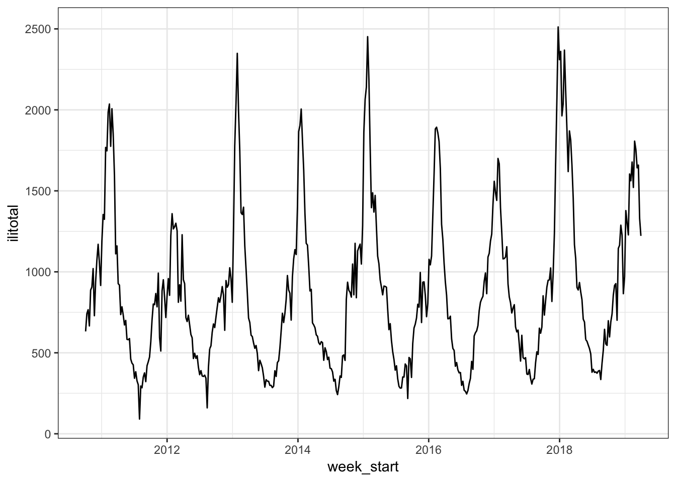
We will hold out 2019 data (13 weeks worth) for testing. The baseline model will use smooth functions of year and week as inputs.

old_model <- gam(ilitotal ~ s(year) + s(week), data = flu_train)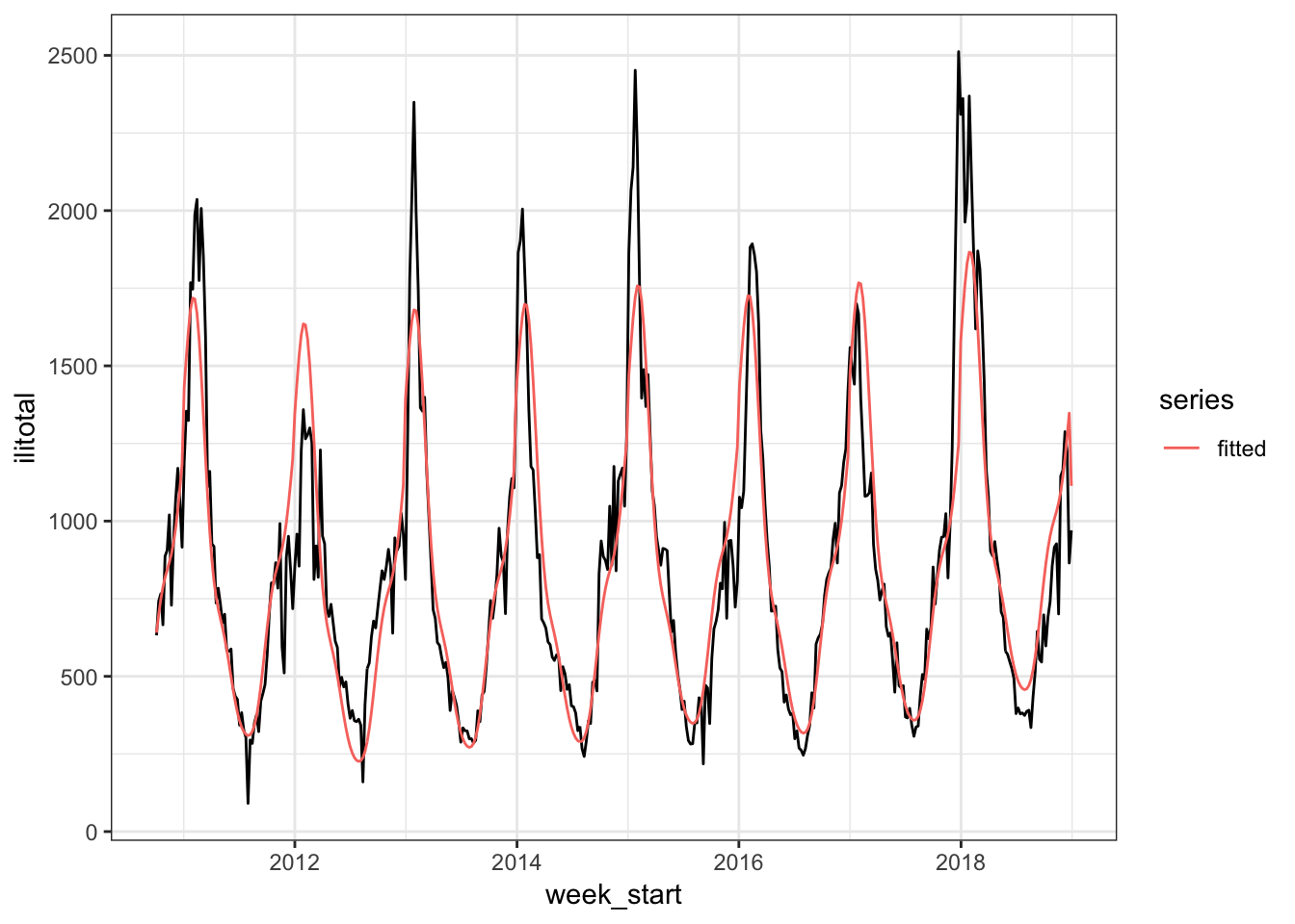

The model is overestimating the peak in the 2012 season and underestimating the peak of the other seasons. Also note how it drops down at the end. If we make forecasts with this model, this drop off will continue but the actual series increases. So this model isn’t very good and our goal to improve upon it.

Different Basis Functions

To improve upon the baseline model one thing we could do is use different basis functions for the smooths. In Gavin Simpson’s post he suggests models of the form \[ y = f_{trend}(x_1) + f_{seasonal}(x_2) \] where we have a smooth to account for the trend component of the series and another smooth to account for the seasonal component. Since the flu data is weekly, we will be using week for our seasonal component. For the trend component we have a couple of options. We could use 1, 2, 3, … as we did before, or as Gavin suggests the data converted to a numeric value. The point is that the variable used for the trend component should capture the overall order of the series. Week represents order only within each year so we need something else to reflect the overall order. We will use the date converted to a numeric value. In R, this gives us the time in days since Jan 1, 1970.

In Gavin’s post he uses the default thin plate spline for the trend variable. However, Noam’s slides suggest considering a Gaussian process smooth. We will try both of these methods.

To model the seasonality of the data we will use what is called a cyclic cubic spline basis. This is like a cubic spline but restricted so that the values at each end of the spline are the same. This should give us continuity between seasons as the end of one seasonal period will match up with the start of the next seasonal period.

Let’s go ahead and fit two models. Both will use a numeric version of time for the trend but one will use a thin plate spline and the other will use a Gaussian process smooth. For the seasonal component we will use a cyclic smooth and additionally specify that we want a basis dimension of 52 which is approximately the number of weeks in a year.

flu_train <- flu_train %>% 
  mutate(time = as.numeric(week_start))

flu_test <- flu_test %>% 
  mutate(time = as.numeric(week_start))

tp_cc <- gam(ilitotal ~ s(time) + s(week, bs = "cc", k = 52),
             data = flu_train)
gp_cc <- gam(ilitotal ~ s(time, bs = "gp") + s(week, bs = "cc", k = 52),
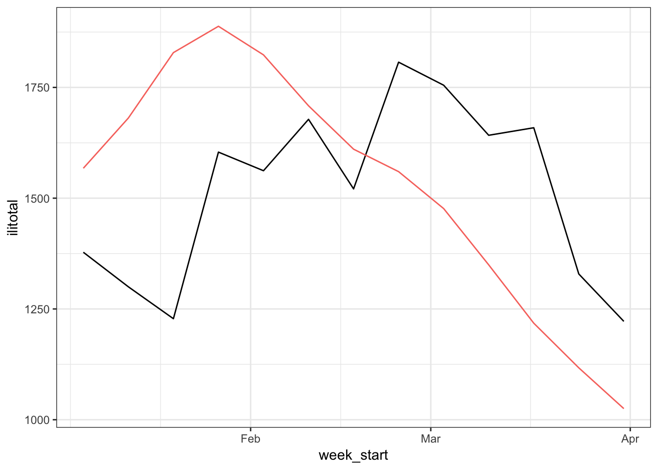
             data = flu_train)

We can see how they are doing compared to our baseline by looking at the fitted values,

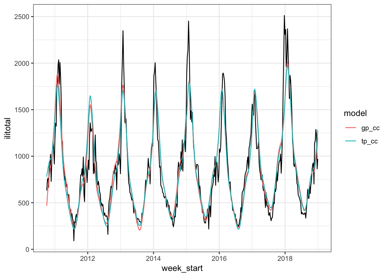
and by looking at the forecasts,

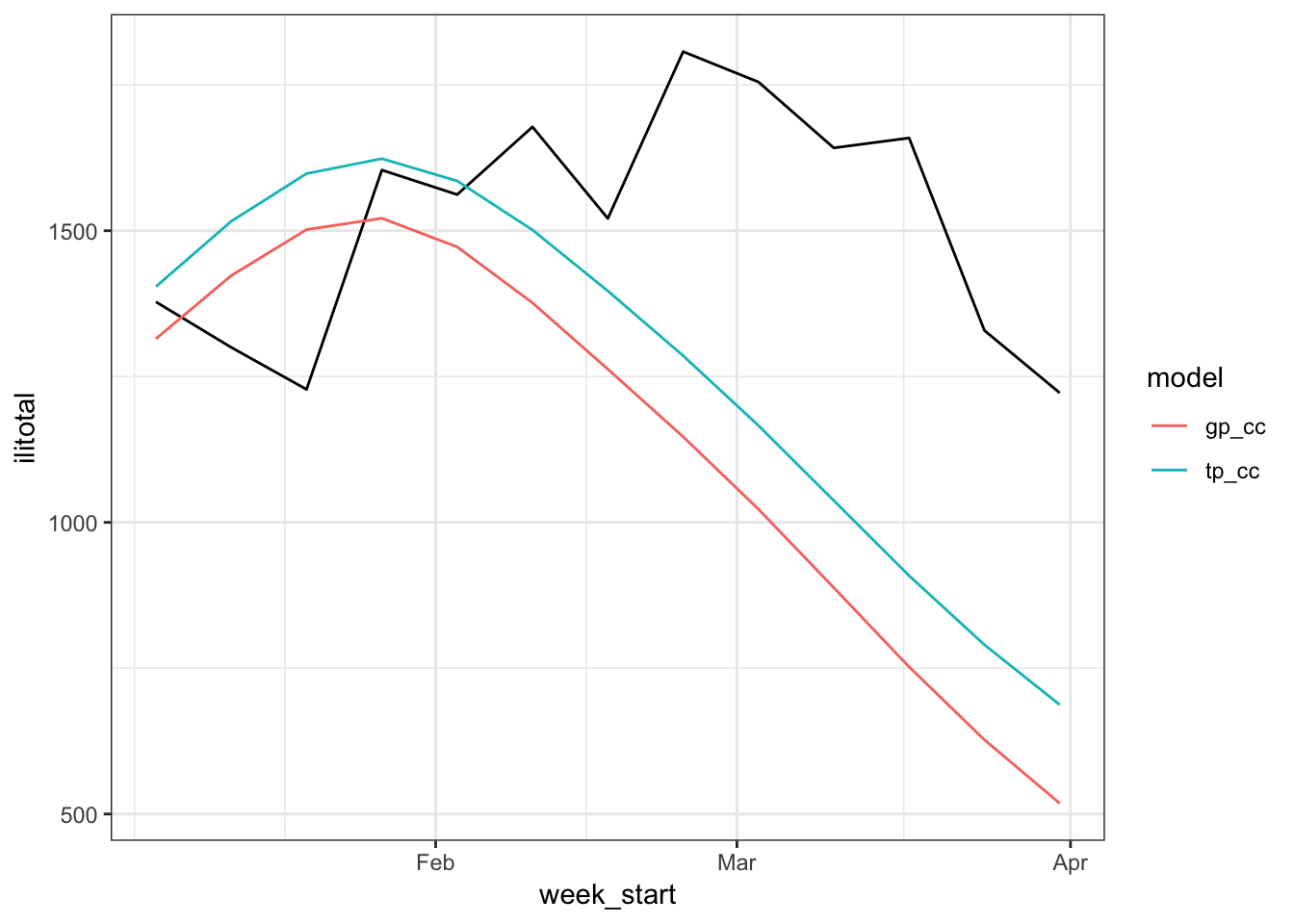
which aren’t very good. One problem might be that we have some residual autocorrelation because we aren’t explicitly accounting for it.

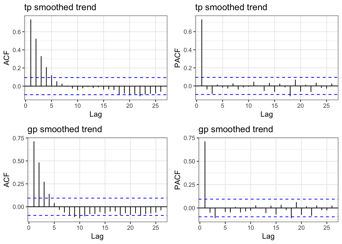
It appears that is the problem. So let’s try to fix it.

Aside - The gratia Package

Before we do that I want to briefly mention the gratia package. gratia is a package by Gavin Simpson that provides ggplot2 based graphics for mgcv objects along with some other helper functions. It’s still a work in progress so not all mgcv model types are supported yet. As an example, we will look at the smooths for the model with the Gaussian process trend smooth.

draw(gp_cc)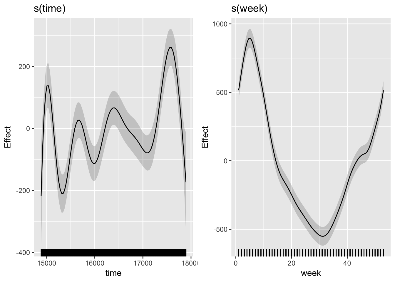

We are using s(time) as our trend component and it seems to be capturing those changes maybe with a bit too much wiggliness. If we look at the original series (above), we see that the peak part of each season rises and falls through the years. The s(week) smooth makes sense as well because it’s high in the early weeks, drops in the summer weeks, and rises again as winter sets in. Also note that the ends of the smooth align because we are using a cyclic cubic spline basis.

Accounting for autocorrelation

The models so far are not so great. Our suspicion is that this is because we aren’t incorporating autocorrelation which is confirmed by the residual plots. We can try to fix that by using the gamm function. The extra ‘m’ is for ‘mixed’ as in a generalized additive mixed model where the mixed model part is used on the residuals. This allows us to specify a correlation structure for the residuals which is exactly what we want.

To keep things from getting too complicated we will stick to the default thin plate spline basis for the trend component. From the ACF and PACF plots, it looks like we should be using AR terms, possibly up to order 4. We specify this in the correlation argument of gamm. First we fit a model as above, without correlated errors so that we can compare models

ar0 <- gamm(ilitotal ~ s(time) + s(week, bs = "cc", k = 52),
            data = flu_train)
ar1 <- gamm(ilitotal ~ s(time) + s(week, bs = "cc", k = 52),
            data = flu_train,
            correlation = corARMA(form = ~ 1|year, p = 1))

ar2 <- gamm(ilitotal ~ s(time) + s(week, bs = "cc", k = 52),
            data = flu_train,
            correlation = corARMA(form = ~ 1|year, p = 2))

ar3 <- gamm(ilitotal ~ s(time) + s(week, bs = "cc", k = 52),
            data = flu_train,
            correlation = corARMA(form = ~ 1|year, p = 3))

ar4 <- gamm(ilitotal ~ s(time) + s(week, bs = "cc", k = 52),
            data = flu_train,
            correlation = corARMA(form = ~ 1|year, p = 4))

Let’s see how the fitted values look.

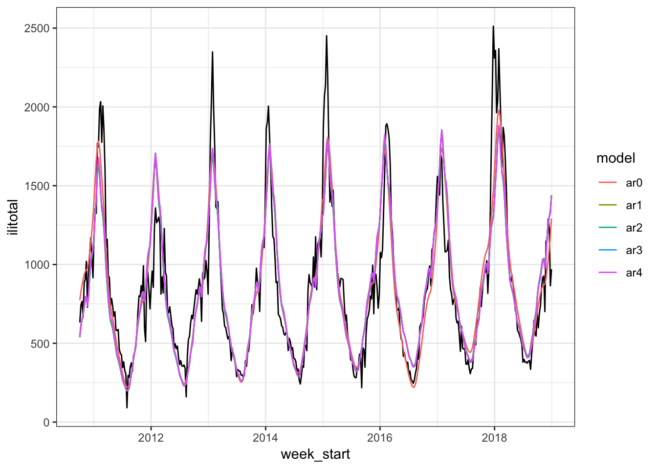
The models look fairly similar and some are a bit hard to tell apart. We can also compare them by using an anova.

anova(ar0$lme, ar1$lme, ar2$lme, ar3$lme, ar4$lme)

##         Model df      AIC      BIC    logLik   Test  L.Ratio p-value
## ar0$lme     1  5 5853.890 5874.221 -2921.945                        
## ar1$lme     2  6 5485.171 5509.568 -2736.586 1 vs 2 370.7186  <.0001
## ar2$lme     3  7 5487.087 5515.549 -2736.543 2 vs 3   0.0848  0.7709
## ar3$lme     4  8 5475.866 5508.395 -2729.933 3 vs 4  13.2208  0.0003
## ar4$lme     5  9 5477.765 5514.360 -2729.883 4 vs 5   0.1007  0.7510

From the AIC and p-values, it looks like we should go with the model with AR(1) residuals. But first let’s see what the residuals look like.

This is much better than we had before. Even though the fitted values don’t look particularly great, we can be more confident with this model. But how do the forecasts look?

Again, these forecasts are not very impressive. What’s going on here? I’m speculating a bit but I think the problem is the predictions don’t involve the AR process we used to model the error terms. Actually, the mgcv documentation says “Prediction from the returned gam object is straightforward using predict.gam, but this will set the random effects to zero.” So basically, the predictions we can get are based on the smooth terms of the gam object and the residual AR process has no effect on the predictions. This is not really a problem if we only cared about the model itself but it does mean that we can’t generate forecasts that incorporate both parts of the model. At least, that’s what I can gather. If you have a way to include both aspects of the model please let me know.

Accounting for autocorrelation - Manually

The only way I could think of to get out of this forecasting pickle was to ‘manually’ fit an ARIMA to the GAM model errors instead of having gamm do it. Fitting a model in this two-stage fashion allows us to generate forecasts of the errors from the ARIMA model and then add them to the predictions from the GAM model to get final forecasts. Really we could use any time series model for the errors but the forecast package has an automatic ARIMA selection function which makes things a lot easier.

gam_mod <- gam(ilitotal ~ s(time) + s(week, bs = "cc", k = 52),
               data = flu_train)

gam_errors <- residuals(gam_mod, type = "response")

error_mod <- auto.arima(gam_errors)
error_mod

## Series: gam_errors 
## ARIMA(1,0,0) with zero mean 
## 
## Coefficients:
##          ar1
##       0.7396
## s.e.  0.0324
## 
## sigma^2 estimated as 16661:  log likelihood=-2706.3
## AIC=5416.6   AICc=5416.63   BIC=5424.73

The auto.arima function chose an AR(1) which makes since considering the previous model. We can also check the residuals to make sure everything is good.

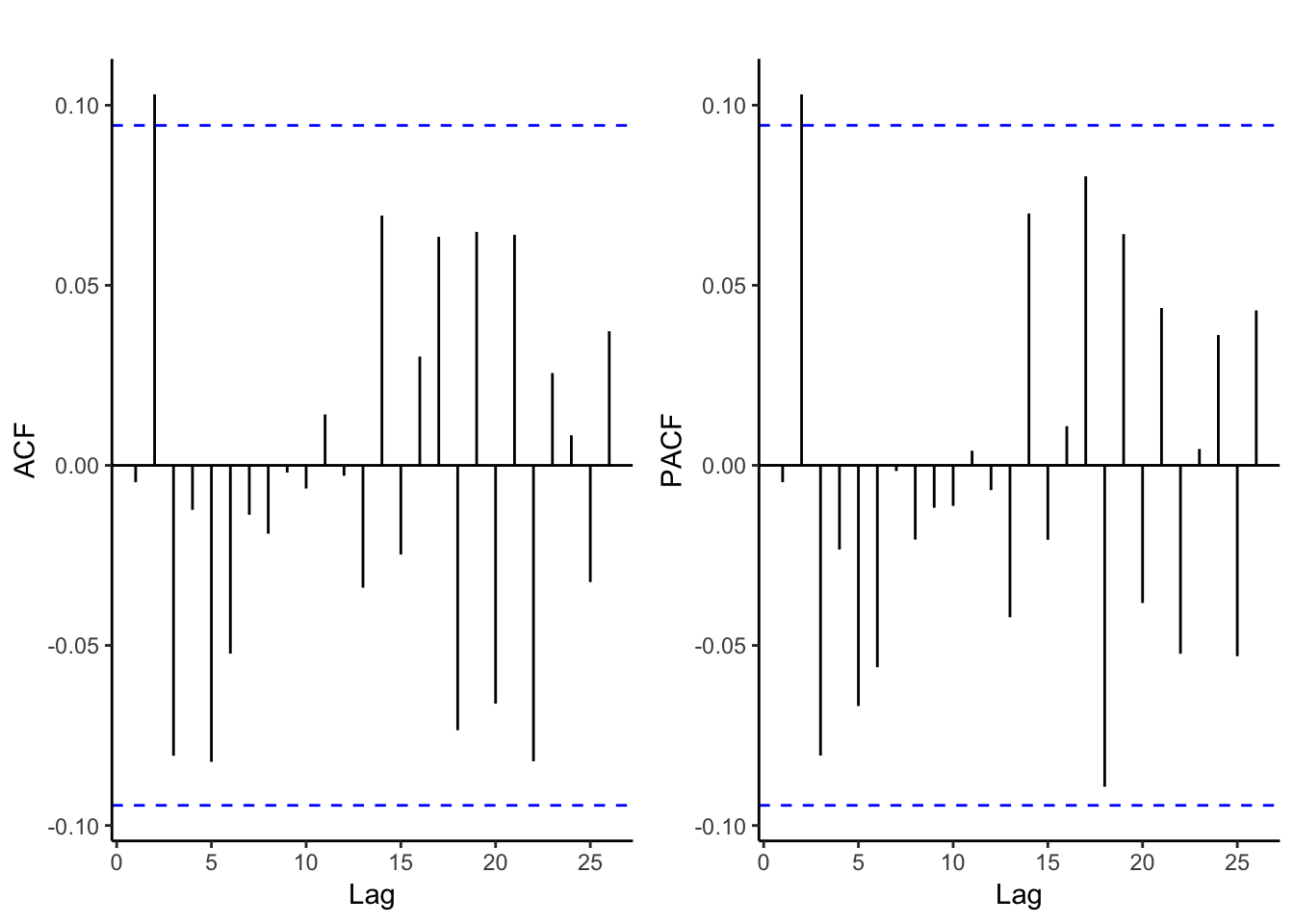
checkresiduals(error_mod, theme = theme_bw())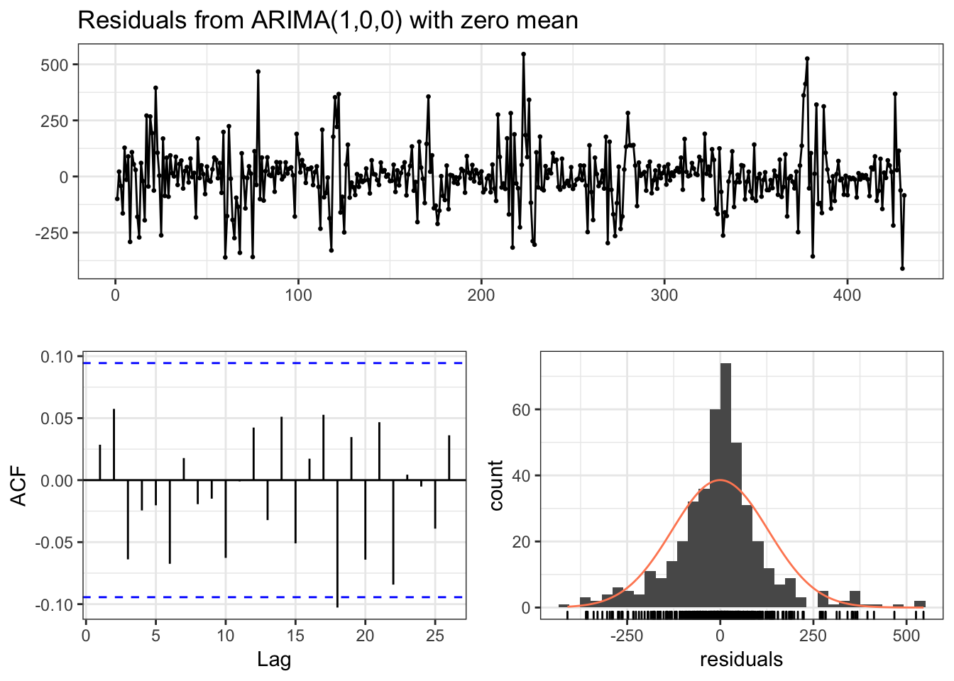

## 
##  Ljung-Box test
## 
## data:  Residuals from ARIMA(1,0,0) with zero mean
## Q* = 8.1562, df = 9, p-value = 0.5185
## 
## Model df: 1.   Total lags used: 10

Good enough for our purposes. Let’s go ahead and generate the forecasts.

error_fcast <- forecast(error_mod, h = 13)$mean
gam_fcast <- predict(gam_mod, newdata = flu_test)
fcast <- gam_fcast + error_fcast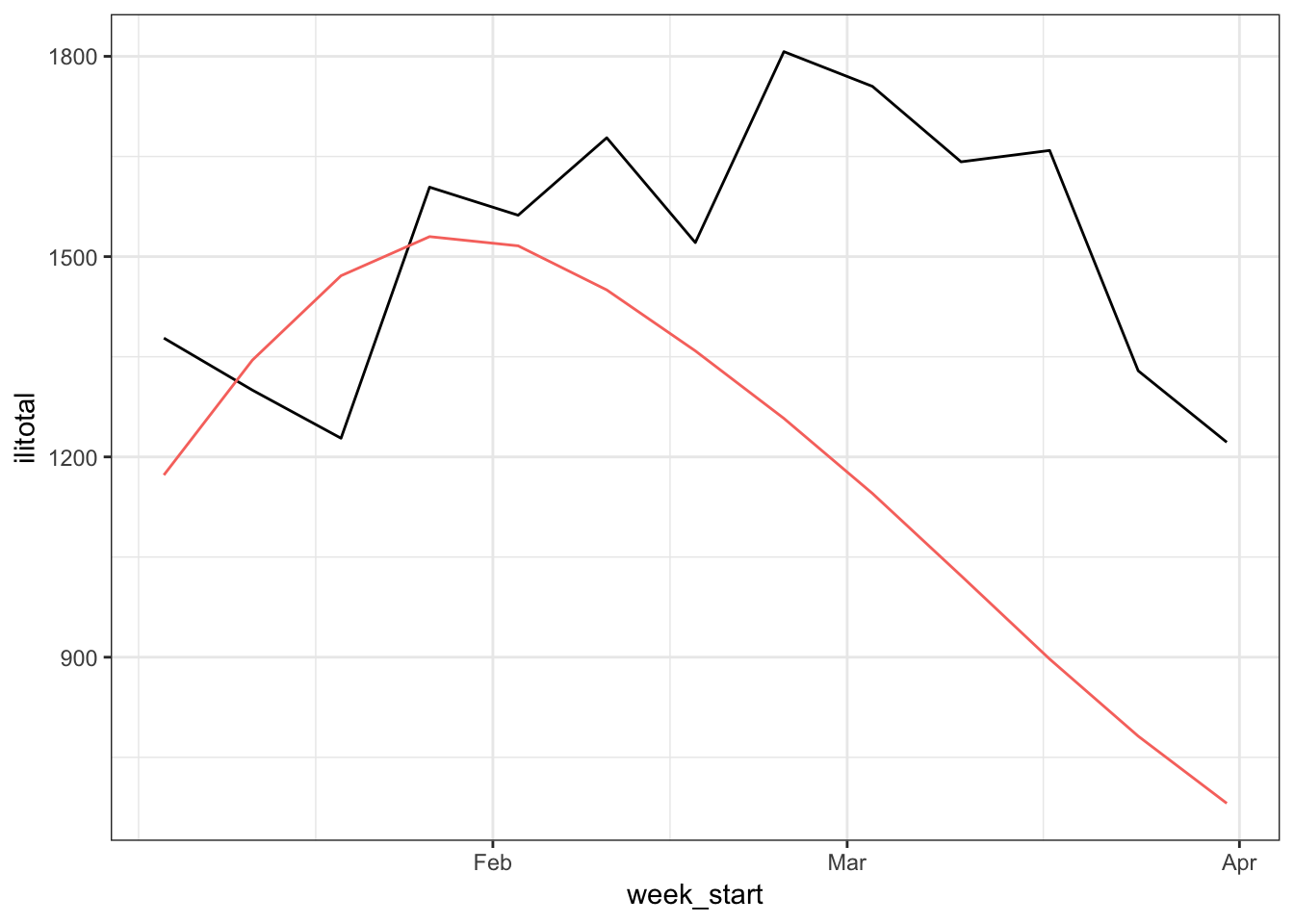

Well this is a bit disappointing. The forecasts are better in the early weeks but like the previous models the downward shift is predicted to happen too soon.

Is there anything else we could have done? Probably, but I’m not sure it would have helped. For example, we could have added in another smooth term interacting time with week. Or even tried different smooths for time and week. Or something besides an ARIMA for the errors. But realistically I think this data is not amenable to this type of modeling scheme. What I mean by that is using smooth functions of time and week to capture trend and seasonality which is a more traditional time series approach. Last time we were able to get good forecasts by just using a few weeks worth of lagged predictors. It seems like that’s the way to go with this data set.