Time Series with Spline Based Models

The Data

The data we will be using comes from the CDC FluView which is a CDC website that has information on influenza in the United States. They also have FluView Interactive, a web application that allows you to interact with flu related data as well as download data.

We will be focusing on the weekly number of influenza-like illnesses (ILI) reported in California from October 2010 to March 2019. The ILI reports come from members of the US Outpatient Influenza-like Illness Surveillance Network, or ILINet. You can download the data from the FluView Interactive website. However, I recommend using the cdcfluview R package which you can find on CRAN or GitHub. The specific data set we will use here is a simplified version and can be found here.

Let’s load the packages we will need and take a quick look at the data. We also add a time index t which we will use later.

library(tidyverse)
library(fields)
library(earth)
library(mgcv)
library(forecast)

theme_set(theme_bw())

flu <- read_csv("https://raw.githubusercontent.com/asbates/nonlinear-models/master/data/ilinet-calif-up-to-2019-03-31.csv") %>% 
  mutate(t = 1:nrow(.))

flu

## # A tibble: 444 x 8
##    week_start  year  week unweighted_ili ilitotal num_of_providers
##    <date>     <dbl> <dbl>          <dbl>    <dbl>            <dbl>
##  1 2010-10-03  2010    40           1.95      632              112
##  2 2010-10-10  2010    41           2.15      742              122
##  3 2010-10-17  2010    42           2.24      766              126
##  4 2010-10-24  2010    43           1.92      666              130
##  5 2010-10-31  2010    44           2.52      887              131
##  6 2010-11-07  2010    45           2.75      906              126
##  7 2010-11-14  2010    46           2.82     1020              131
##  8 2010-11-21  2010    47           3.16      729              134
##  9 2010-11-28  2010    48           2.61      939              135
## 10 2010-12-05  2010    49           3.06     1072              135
## # … with 434 more rows, and 2 more variables: total_patients <dbl>,
## #   t <int>

The data starts at week 40 of 2010 which is October 03. The column of interest for us is ilitotal which is the total number of reported patients with flu-like illnesses. Let’s look at a time plot of the series.

flu %>% 
  ggplot(aes(week_start, ilitotal)) +
  geom_line()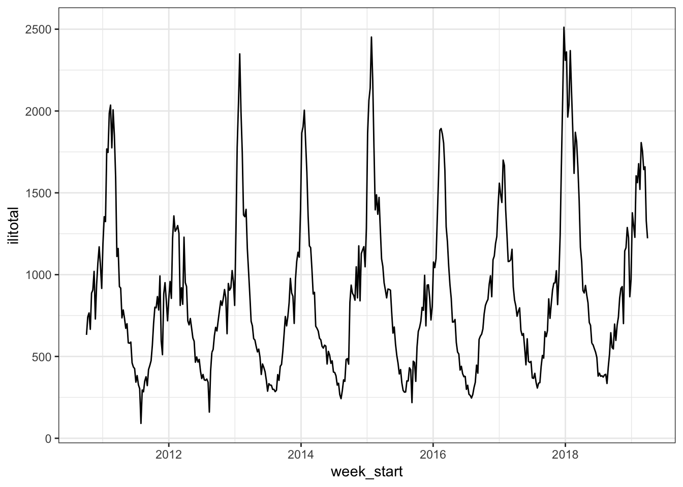

Unsurprisingly there is some obvious seasonality with more reported cases in the winter months.

First Approach

For our first approach at modeling we will use time indexed as \(t = 1, 2, 3, ..., n\). This is the simplest approach and is the default behavior of the ts class in R. Before we start modeling though, we will do setup. First we will use 2019 data as a holdout set. The last observation in this data is for the week of March 31 so this gives us 3 months for testing (13 weeks). We will also use an ARIMA for comparison so we will create a ts version of the data. Lastly, the Tps function we will use for the thin plate spline takes an \(x/y\) pair instead of a formula and data frame so we will need to create those as well.

flu_train <- filter(flu, week_start < "2019-01-01")
flu_test <- filter(flu, week_start >= "2019-01-01")

flu_ts <- ts(flu$ilitotal, frequency = 52)
flu_ts_train <- flu_ts[1:nrow(flu_train)]
flu_ts_test <- flu_ts[(nrow(flu_train) + 1):nrow(flu)]

# Tps requires x/y
x_train <- flu_train %>%
  select(t)

y_train <- flu_train %>% 
  select(ilitotal)

x_test <- flu_test %>% 
  select(t)

y_test <- flu_test %>% 
  select(ilitotal)

Now we are ready to go with model fitting.

# ARIMA
arima_mod <- auto.arima(flu_ts_train)

# thin plate spline
tps_mod <- Tps(x_train, y_train)

# MARS
mars_mod <- earth(ilitotal ~ t, data = flu_train)

# GAM
gam_mod <- gam(ilitotal ~ s(t), data = flu_train, method = "REML")

If this was a ‘real’ analysis we would of course want to investigate the fit of these models by looking at the estimated parameters, residuals, etc. But for our purposes we will just be considering the forecasts to keep things simple. First let’s see how well each of the models fits the training data.

flu_train <- flu_train %>% 
  mutate(
    fitted_arima = fitted(arima_mod),
    fitted_tps = fitted(tps_mod)[,1],
    fitted_mars = predict(mars_mod)[,1],
    fitted_gam = fitted(gam_mod)
  )


flu_train %>% 
  select(week_start, ilitotal, starts_with("fitted")) %>% 
  gather("model", "value", -week_start, -ilitotal) %>% 
  mutate(model = str_remove(model, "fitted_")) %>% 
  ggplot(aes(week_start, ilitotal)) +
  geom_line() +
  geom_line(aes(y = value, color = model))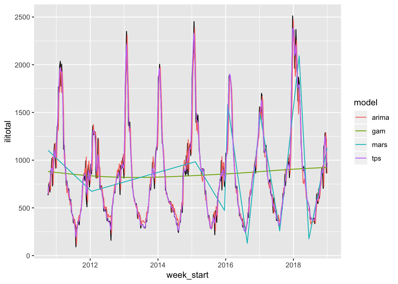

The MARS and GAM are obviously doing poorly. This is likely due to the way we specified the time index because, as we will see shortly, they look much better using other approaches. The ARIMA and thin plate spline are doing the best so let’s see how well they do on the test set.

flu_test <- flu_test %>% 
  mutate(
    pred_arima = forecast(arima_mod, h = 13)$mean[1:13],
    pred_tps = predict(tps_mod, x_test)[,1]
  )

flu_test %>% 
  select(week_start, ilitotal, starts_with("pred")) %>% 
  gather("model", "forecast", -week_start, -ilitotal) %>% 
  mutate(model = str_remove(model, "pred_")) %>% 
  ggplot(aes(week_start, ilitotal)) +
  geom_line() +
  geom_line(aes(y = forecast, color = model))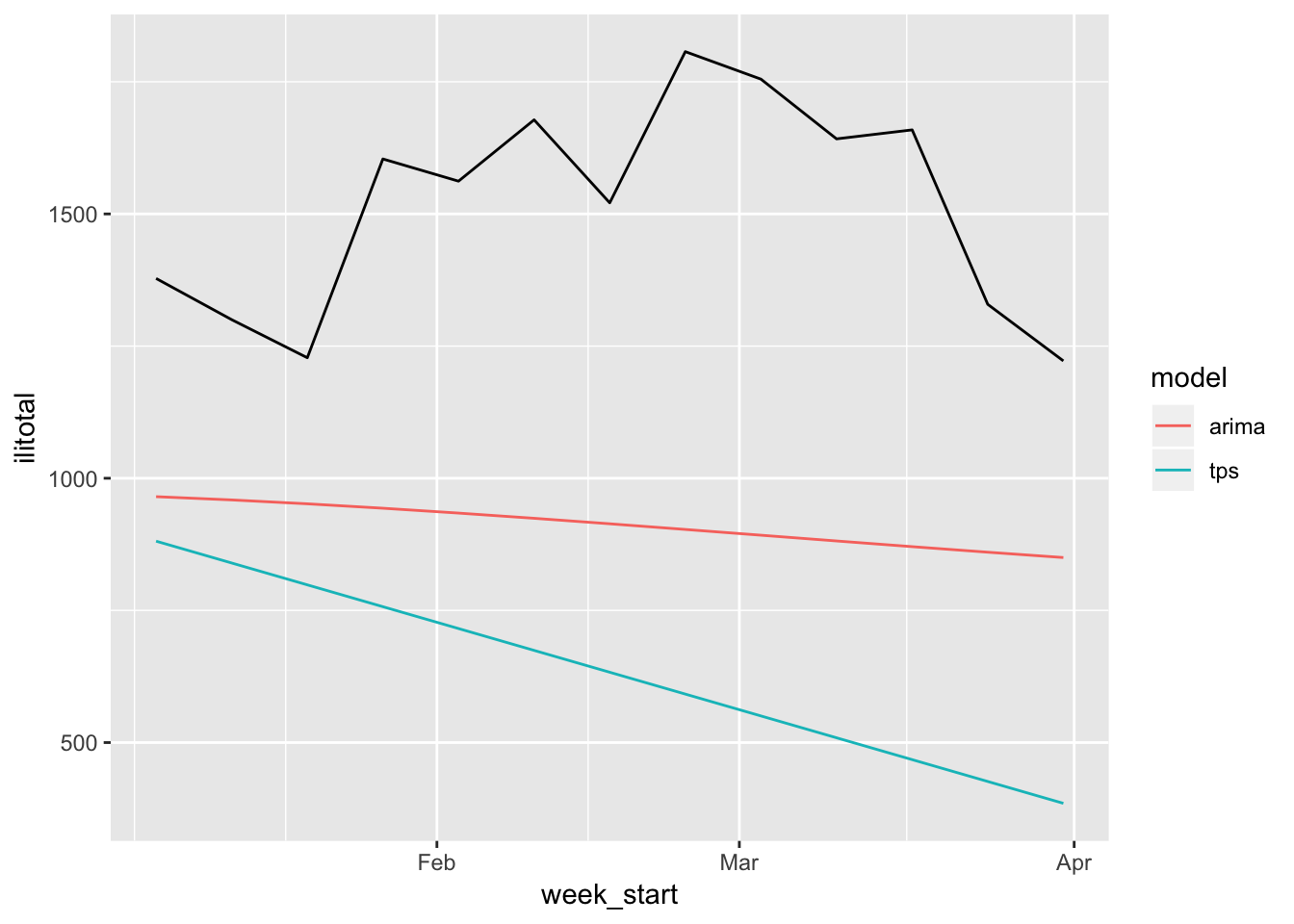

These don’t look so great. We can plot the original data along with these forecasts to get a better sense of just how far off they are.

flu %>%
  ggplot(aes(week_start, ilitotal)) +
  geom_line() +
  geom_line(aes(week_start, pred_arima, color = "blue"), data = flu_test) +
  geom_line(aes(week_start, pred_tps, color = "red"), data = flu_test) +
  scale_color_discrete(name = "model", labels = c("arima", "tps"))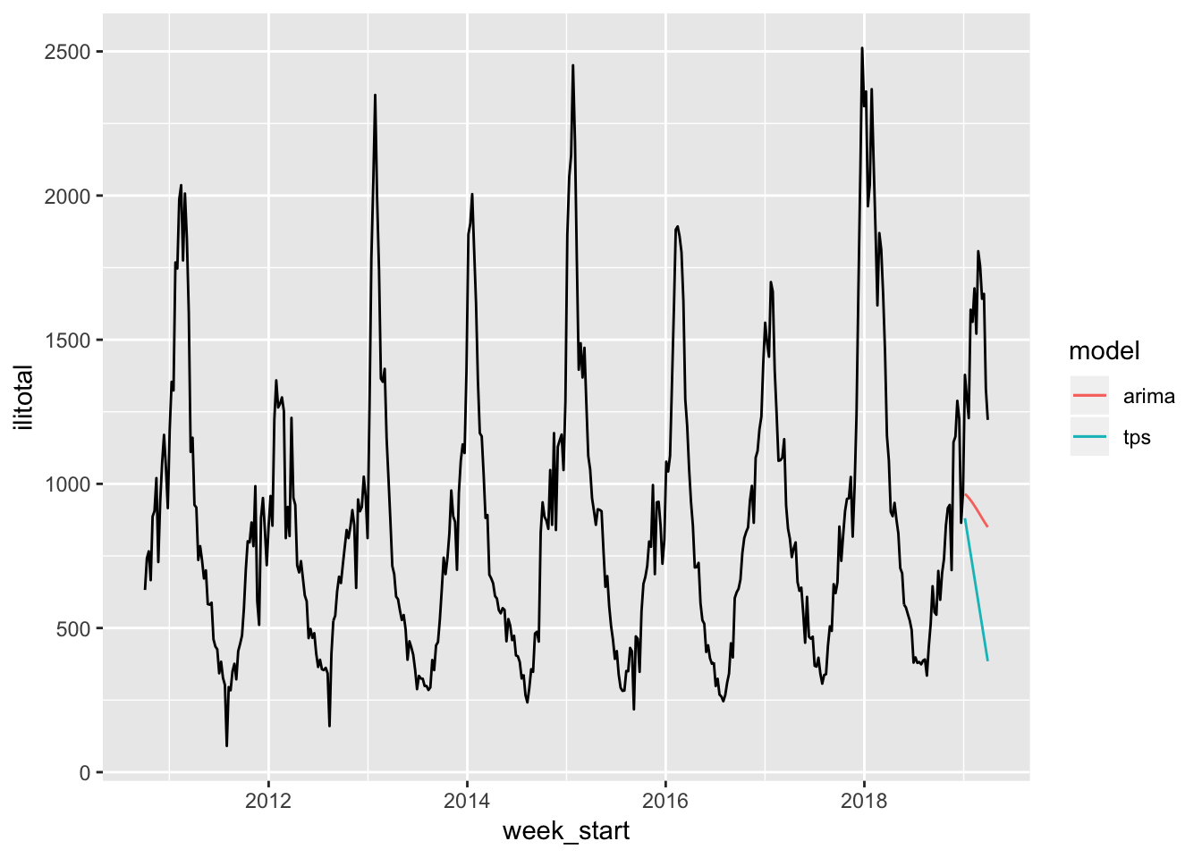

Yes, terrible.

Second Approach

Now we will see how things change when we use the year and week as the time index instead of \(1, 2, ..., n\). This makes more sense for this data because the number of flu-like illnesses in say weeks 3 and 50 will be a lot different than in week 20. The code is almost the same as before so I won’t show most of it. If you’re interested you can find it here. The only real difference is the model specification.

tps_mod <- Tps(x_train, y_train)
mars_mod <- earth(ilitotal ~ year + week, data = flu_train)
gam_mod <- gam(ilitotal ~ s(year) + s(week), data = flu_train, method = "REML")

This time x_train has two columns, year and week, and we use a separate smooth for year and week in the GAM¹. We don’t use the ARIMA model here because it won’t change and we already saw how poor the forecasts were.

Let’s see how the models fare using this approach by first looking at the fitted values.

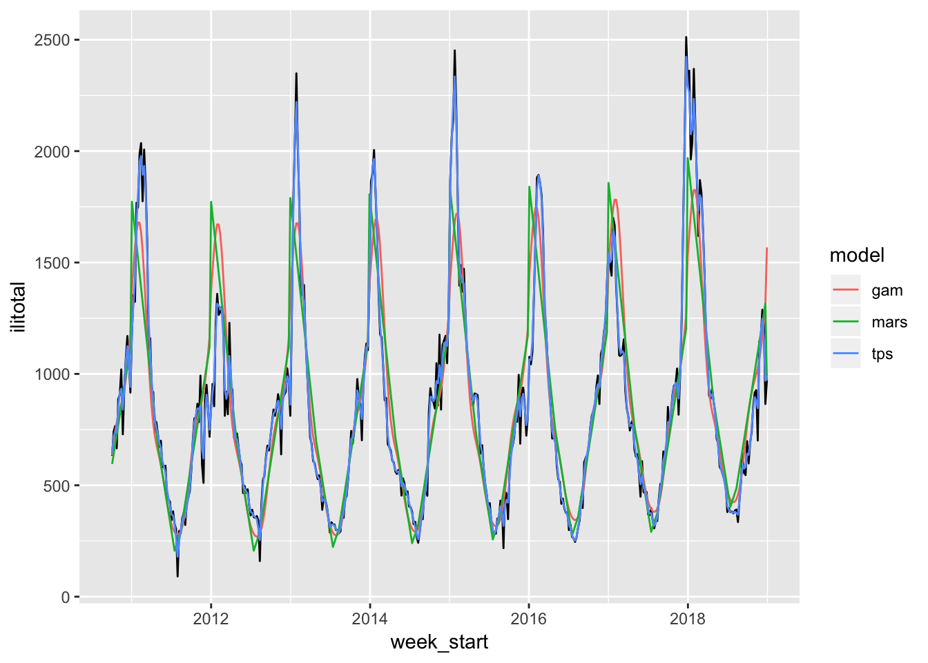
The MARS and GAM models do much better here although still not quite as good as the thin plate spline. Let’s see how each of their forecasts do.

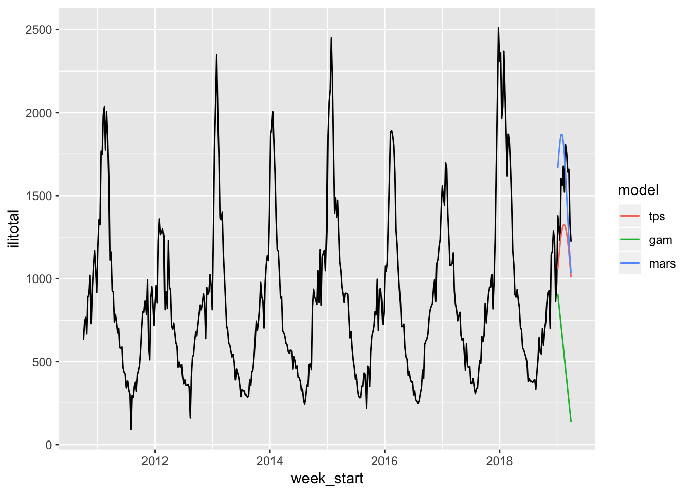
The thin plate spline is much better this time around. The MARS and GAM are still lacking.

Third Approach

This time we will use lagged values of the series as predictors instead of time. We will use four lags. For the GAM we use a separate smooth for each lag and no interactions between them.

flu <- flu %>% 
  mutate(
    lag_ilitotal = lag(ilitotal),
    lag2_ilitotal = lag(ilitotal, n = 2L),
    lag3_ilitotal = lag(ilitotal, n = 3L),
    lag4_ilitotal = lag(ilitotal, n = 4L)
  )

Again, let’s see how well the models fit the training set.

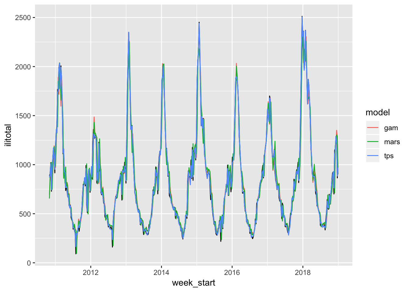
Clearly the MARS and GAM are having a much easier time now. Actually all of the models seem to be doing quite well. It’s a bit hard to see the original series in black. But the real test is the forecasts…

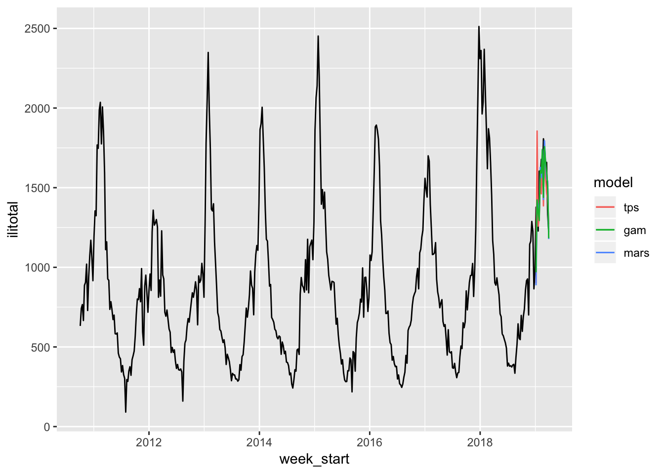
The MARS and GAM really come into their own now. Their forecasts actually look better than the thin plate spline which has a large spike above the actual data. It’s hard to tell a difference between the MARS and GAM visually so let’s look at a numeric summary of their fit.

yardstick::metrics(flu_test, truth = ilitotal, estimate = pred_gam)

## # A tibble: 3 x 3
##   .metric .estimator .estimate
##   <chr>   <chr>          <dbl>
## 1 rmse    standard     220.   
## 2 rsq     standard       0.259
## 3 mae     standard     171.

yardstick::metrics(flu_test, truth = ilitotal, estimate = pred_mars)

## # A tibble: 3 x 3
##   .metric .estimator .estimate
##   <chr>   <chr>          <dbl>
## 1 rmse    standard     201.   
## 2 rsq     standard       0.306
## 3 mae     standard     153.

Based on this I would go with the MARS model if I had to pick one.

Next Steps

Let’s take a minute to talk about other things we might do if we wanted to take this further. Like I mentioned before we should probably look at model diagnostics to help decide on which model we would want to use. Another thing we could do is a time series cross validation. This is where we slide along the series using only a portion of the data at a time. For example we could use the first two months for training and the third month to test our forecasts. Then months two and three become the training data, month four the testing data, and so on. This would give us a better indication of how well our model would hold up over time. Maybe we just got lucky by only looking at the last month of the series. We would also want to compute forecast intervals. The MARS model is giving better point forecasts but maybe the GAM gives us better forecast intervals in which case we would go with the GAM. Note that this would probably require a time series bootstrap because I don’t think there is any way to get forecast intervals for MARS or GAM models.

The End

Hopefully this gives you a feel for how to model time series with models that aren’t time series models per se. I was fairly unsure how to apply the models I’ve learned so far in my course to time series so I learned a lot in developing this post.