As you may have guessed from the title of the post, we are going to talk about multivariate adaptive regression splines, or MARS. MARS is multivariate spline method (obviously) that can handle a large number of inputs.
Multivariate spline methods can have some problems with a high dimensional input \(x\). Why? Because the size of the basis grows exponentially with the number of inputs. Suppose we have two inputs, \(x_1\) and \(x_2\), along with a set of basis functions \(h_{1k}(x_1), k = 1, 2, ..., M_1\) for \(x_1\) and basis functions \(h_{2k}(x_2), k = 1, 2, ..., M_2\) for \(x_2\). These can be any sort of spline basis functions. For example, each of the \(h\)s can define a natural spline basis. To estimate our function \(f\), we combine these two bases together multiplicatively to get \[ g_{jk}(x) = h_{1j}(x_1)h_{2k}(x_2) \] where \(j\) runs from 1 to \(M_1\) and \(k\) runs from 1 to \(M_2\). This defines what is called a tensor product basis for \(f\) which looks like \[ f(x) = \sum_{j=1}^{M_1} \sum_{k = 1}^{M_2} \beta_{jk}g_{jk}(x). \] The number of basis functions grows extremely fast. To see this, imagine we want to use cubic splines with two knots for each \(x\). In this case there are 6 basis functions for \(x_1\) and 6 basis functions for \(x_2\). When we combine these to get a basis for \(f\), we get 36 (\(6^2\)) basis functions \(g_{jk}\) because we multiply each of the basis functions \(h_{1k}\) for \(x_1\) with each of the functions \(h_{2k}\) for \(x_2\). Three inputs would give \(6^3\) or 216 basis functions for \(f\). Wow! We went from 6 to 216 just by adding two more variables. And this is assuming only two knots for each \(x_i\). In reality we would likely have more knots thus more basis functions and the numbers would be even bigger. MARS attempts to remedy this by considering, but not including, all possible basis functions for each \(x_i\). But before we get into that, let’s see what kind of basis functions MARS uses.
MARS Basis Functions
MARS uses linear splines as basis functions. These take the form \(h(x) = (x-t)_{+}\) where \(t\) is a knot and the \(+\) means the positive part. That is, \[ (x - t)_{+} = \begin{cases} x - t &\text{ if } x > t \\ 0 &\text{ if } x \le t. \end{cases} \] This is similar to the truncated-power basis we saw previously with order \(M = 2\). The difference is that for MARS we don’t include the \(x\) term, just the intercept and \((x - t)_{+}\) terms. Actually, the basis functions for MARS come in pairs: \((x-t)_{+}\) and \((t-x)_{+}\).
For the knots, we use the unique values of each \(x_j\). This gives quite a bit of basis functions but as we will see soon not all of them will be included in the final model. With these knots and the truncated linear basis functions, the entire1 basis for \(f\) is the set \(B = \{ (x_j - t)_{+}, (t-x_j)_{+} \}\) where \(t\) takes values in \(\{ x_{1j}, x_{2j}, ..., x_{nj}\}\) and \(j\) runs from 1 to \(p\).
MARS Model Fitting Procedure
The MARS fitting procedure is is a two stage process. The forward stage is the same idea as forward stepwise regression. This could result in a large number of terms and overfitting so the backwards stage tries to mitigate this be dropping some terms.
The Foward Step
The forward stage of the fitting procedure starts by including only the constant (or intercept) term. We then consider adding each function in \(B\) pairwise and pick the pair that reduces the error the most. Next, we try adding product terms, selecting again from the candidate pairs in \(B\) and choosing the pair that minimizes the error. This process is continued until a predefined number of terms are included. Suppose we have a function \(h_{\ell}(x)\) already included in the model (\(h_{\ell}\) could be 1 or something like \((x-t)_{+}\) or \((x_1-t_1)_{+} (x_2-t_2)_{+}\)) and there are \(k\) such terms. Then we consider expanding the model by adding two terms, \[ \hat{\beta}_{k+1}h_{\ell}(x)(x_j-t)_{+} + \hat{\beta}_{k+2}h_{\ell}(x)(t-x_j)_{+}, \] and keeping the pair with the smallest error.
Let’s run through an example to illustrate this idea. First, we include the intercept 1, and this is our entire model. Now suppose we look at all the choices and find that we want to include the variable \(X_3\) with a knot at \(x_{23}\), the second value for \(X_3\), because this results in the lowest error. Now our model looks like \[ \beta_0 + \beta_1 (X_3-x_{33})_{+} + \beta_2 (x_{33} - X_3)_{+}. \] At this stage we have three \(h\)s in the model: \(h_0(x)= 1, h_1(x) = (X_3-x_{33})_{+}\), and \(h_2(x) = (x_{33} - X_3)_{+}\). Next, we consider multiplying one of the functions in \(B\) by one of the three \(h\)s already included in our model. We might find that we want to include \((X_2 - x_{27})_{+}\) and \((x_{27} - X_2)_{+}\), the second variable with a knot at the 7th value of this variable. Specifically, we want to include this pair with \(h_0(x) = 1\). Now are model has the form \[ \beta_0 + \beta_1 (X_3-x_{33})_{+} + \beta_2 (x_{33} - X_3)_{+} + \beta_3(X_2 - x_{27})_{+} + \beta_4(x_{27} - X_2)_{+}. \] If we had decided ahead of time that we wanted to include only 5 terms in our model we would be done. If we wanted more terms we would repeat this process until we get to the desired number of terms.
The Backward Step
For the backward stage of the fitting procedure we simplify the model by deleting terms. The choice of which term to remove is based on which one results in the smallest increase in error upon removal. This gives us a bunch of different models each with a different number of terms. The final model is chosen using generalized cross validation (GCV). We could use regular cross validation too but this is more expensive computationally. We won’t get into the details of GCV here. Basically, we apply a formula to each model (that have different numbers of terms) and pick the best one.
Why Linear Basis Functions?
When I first saw that all the basis functions were linear I wondered why we didn’t include higher powers. Why not follow the same fitting procedure but consider for example \((x-t)_{+}^2\) in addition to the linear terms? Apparently there is a good reason for this that Hastie and friends discuss in The Elements of Statistical Learning. When the MARS basis functions are multiplied together, they are only nonzero over a small part of the input space and zero everywhere else. So the regression surface is nonzero only when it needs to be. Higher order polynomial products however, would give a surface that is nonzero everywhere which apparently wouldn’t work as well. The zeroness of the linear basis function products also has the effect of saving parameters as we only need parameters in the nonzero parts. With a high dimensional input space this is especially important. As usual, there are also computational reasons but we won’t worry about them here.
An Example
Let’s look at an example. Previously we made up some data so we could see how fitted models compared to their truths and didn’t look into the model fitting packages much. This time we will focus on getting familiar with the R package earth, which implements MARS. The data we will use is included in the package. ozone1 contains ozone readings from Los Angeles along with several covariates. Let’s start by loading the data and fitting a MARS model:
library(earth)
mars <- earth(O3 ~., data = ozone1)
mars
## Selected 12 of 20 terms, and 9 of 9 predictors
## Termination condition: Reached nk 21
## Importance: temp, humidity, dpg, doy, vh, ibh, vis, ibt, wind
## Number of terms at each degree of interaction: 1 11 (additive model)
## GCV 14.61004 RSS 4172.671 GRSq 0.7730502 RSq 0.8023874It looks like there were 20 model terms under consideration and 12 of them were included in the final model. Termination condition: Reached nk 21 tells us that the forward pass stopped when it reached 21 terms. earth chooses this number based on the number of inputs but we have the option to change it.
What can we do with an earth object?
methods(class = "earth")## [1] anova case.names coef deviance
## [5] effects extractAIC family fitted
## [9] fitted.values format hatvalues model.matrix
## [13] plot plotmo.pairs plotmo.singles plotmo.y
## [17] predict print resid residuals
## [21] summary update variable.names weights
## see '?methods' for accessing help and source codeAs expected we have the usual methods like summary, residuals, etc. Let’s see what plot does.
plot(mars)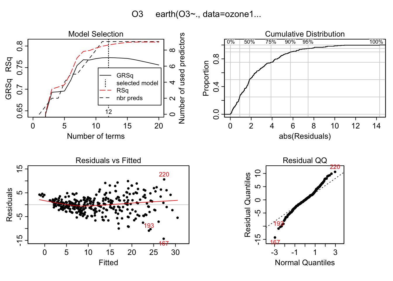 This shouldn’t be surprising. Usually plotting a model objects gives residual plots. We can also get two types of variable importance measures and there is a plotting method for them as well.
evimp(mars)## nsubsets gcv rss
## temp 11 100.0 100.0
## humidity 8 32.0 34.8
## dpg 8 32.0 34.8
## doy 8 32.0 34.8
## vh 7 31.6 33.9
## ibh 5 27.3 29.9
## vis 5 15.3 19.3
## ibt 4 7.9 13.6
## wind 2 5.3 9.4When looking at the methods I was curious about the plotmo methods. After a quick search I found that plotmo is a package for plotting regression surfaces. It’s written by the same person who wrote earth, Stephen Milborrow. Le’s see what it does.
plotmo(mars)## plotmo grid: vh wind humidity temp ibh dpg ibt vis doy
## 5760 5 64 62 2112.5 24 167.5 120 205.5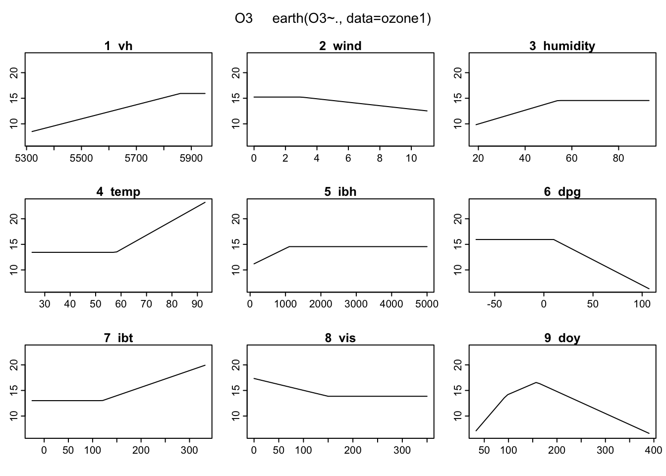 This is pretty cool. It shows us the basis functions for each of the input variables. But the
 plotmo description says it can plot surfaces. After some more digging I figured out how to do this. By default, earth doesn’t include interaction terms like \((x-t)_{+}(x-r)_{+}\). In order to get a surface plot, we need to have interactions because we need two input variables. We can do this by modifying the original model.
# include just 3 variables for simplicity
oz <- ozone1[, c("O3", "wind", "humidity", "temp")]
mars2 <- earth(O3 ~., data = oz, degree = 2) # allow first order interactions
plotmo(mars2)
## plotmo grid: wind humidity temp
## 5 64 62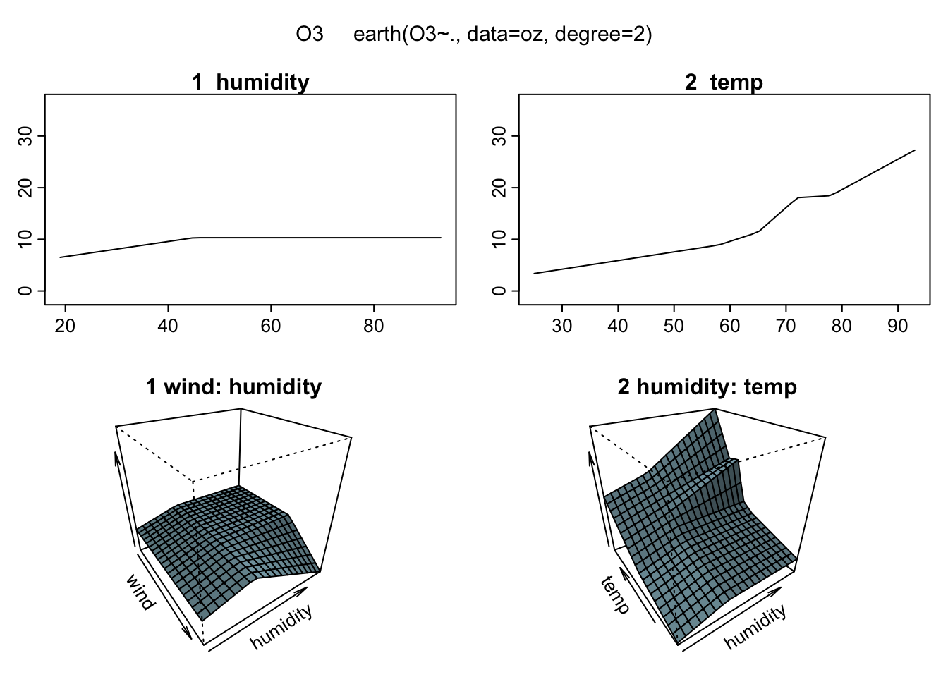 This is fantastic! It let’s actually see how the regression surface is built up instead of just looking at a bunch of error numbers. Unfortunately, unless you live in a higher dimensional world you can’t see the full surface. But for the rest of us this is as close as we can get.
A Few Notes On earth
We just looked at a few features of the earth package here but there is a lot more we could do. For example, the earth function has a bunch of options one could play around with. There is a vignette that goes into more detail about the package that I suggest you take a look at. It gives more detail on the forward and backward passes and some of the limitations of the package (e.g. no missing values). If you like the regression surface plots I recommend you also check out the plotmo vignette Plotting regression surfaces with plotmo.
we also include a constant term.↩