Thin Plate Splines

Multivariate Splines

The simplest approach would be to fit a spline to each of the \(x\)s. For example, if we have \(x_1\) and \(x_2\) then we could fit a spline to \(x_1\) and a spline to \(x_2\). This would make new \(x\) values to which we could fit a linear model to. In R code it would look something like lm(y ~ bs(x1) + bs(x2), data = df) with bs coming from the splines package and a data frame df (we could also add linear terms if we wanted to). We will take a different approach in this post.

Thin Plate Splines

At the core, thin plate splines are a multivariate version of smoothing splines. Remember that smoothing splines are fit by minimizing the residual sum of squares with a smoothness penalty based on the second derivative of the function \(f\) we are trying to approximate: \[ RSS(f, \lambda) = \sum_{i=1}^n (y_i-f(x_i))^2 + \lambda \int [f''(t)]^2 dt. \] So how does this generalize this to higher dimensions? Well, the first part of this term doesn’t change. Even if the inputs to \(f\) are multivariate, the output is still univariate. What needs to be adjusted then is the penalty term. Hopefully it’s not too surprising that instead of a \('\), a univariate derivative, we use a \(\partial\), a partial derivative. And since the penalty term involves a second derivative, we need to look at second partial derivatives. Now that we are in a multivariate setting, there isn’t just “the” second derivative so we need to look at mixed partials as well. So our residual sum of squares will look like \[ RSS(f, \lambda) = \sum_{i=1}^n (y_i-f(x_i))^2 + \lambda J(f) \] as before but with the penalty \[ J(f) = \int \left[ \left(\frac{\partial^2f(x)}{\partial x_1^2} \right)^2 + 2\left(\frac{\partial^2f(x)}{\partial x_1x_2} \right)^2 + \left(\frac{\partial^2f(x)}{\partial x_2^2} \right)^2 \right] dx_1 dx_2. \]

In general, the penalty function \(J\) is \[ J(f) = \int \sum \frac{m!}{\alpha_1! \cdots \alpha_d!} \left(\frac{\partial^m f(x)}{\partial x_1^{\alpha_1} \cdots \partial x_d^{\alpha_d}} \right)^2 dx. \] This is quite a bit more complex that smoothing splines so let’s break this down. \(m\) is the order of the derivatives we take and \(d\) is the dimension of \(x\) (both are 2 in the previous equation). The \(\alpha\)s are non-negative integer vectors such that \(\sum \alpha_i = m\). As an example, suppose \(m = 2\) and \(d = 1\). This means we have a univariate \(x\) and we take second derivatives. The restriction that the \(\alpha\)s sum to \(m\) means that \(\alpha_1 = 2\). Then the penalty function is \[ J(f) = \int \frac{2!}{2!} \left(\frac{\partial^2 f(x)}{\partial x^2} \right)^2 dx. \] But in this case \(x\) is univariate so what we really have is \[ J(f) = \int (f''(x))^2 dx, \] which is the penalty for a cubic smoothing spline.

It’s a bit hard to see (I didn’t work this out myself) but it turns a thin plate spline is a linear function of the response. Similar to what we saw with smoothing splines, there is a smoother matrix \(S_{\lambda}\) that we can use to write the fitted values as \[ \hat{f}(x) = \hat{y} = S_{\lambda}y. \] \(S_{\lambda}\) is analogous to the hat matrix \(H\) in standard linear regression and we can use it to do things like determine the degrees of freedom and obtain the residuals as \((I-S_{\lambda}y)\).

An Example

Alright, enough of this math stuff, let’s look at an example. For this example, I just want to help get a visual of what is going on with these thin plate spline things and demonstrate how to fit one in R. As before, we will use some fake data so we have a truth for comparison.

First we generate some data, a polynomial with some added noise, and then plot it.

library(dplyr)
library(lattice)

set.seed(42)
df <- expand.grid(x = -10:10, y = -10:10) %>% 
  mutate(z = y + x^2 + y^2 - x*y - x^2*y + rnorm(n(), 100, 20))

wireframe(z ~ x*y, df)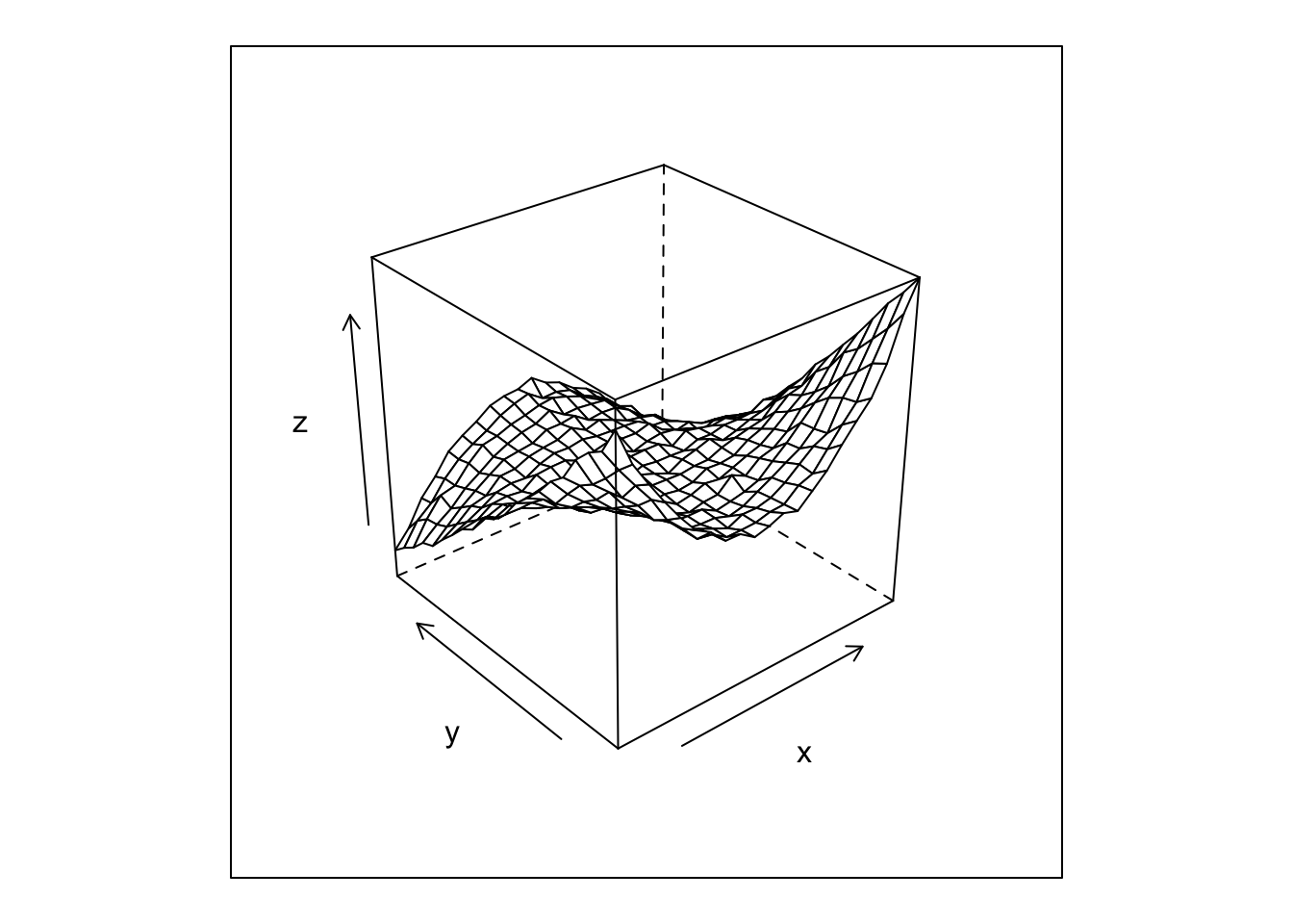

To fit a thin plate spline we are going to use the fields package. Fun fact! fields started out as FUNFITS, a package for S-Plus. Barbara Bailey, my advisory for the nonlinear models self study I’m taking, was one of the authors of FUNFITS. That’s how I heard of the fields package. I think mgcv is a more modern package that can fit thin plate splines. But we will hold off on using it until we start looking at generalized additive models. Anyways, let’s fit a thin plate spline:

library(fields)

# takes x,y instead of formula
model_x <- df %>% select(x,y)
model_y <- df %>% select(z)

fit <- Tps(model_x, model_y)

The model summary is quite hefty so I don’t print it out here. As you might expect it gives things like the degrees of freedom and smoothing parameter. Like most modeling functions there are various arguments for specifying the fitting method, etc. but we won’t get into those here.

To see how well the model fits we can add the fitted values the plot of the data above¹.

pred_tps <- predict(fit)

# add predicted and true values
df <- df %>% 
  mutate(true_z = y + x^2 + y^2 - x*y - x^2*y) %>% 
  mutate(fitted_z = as.vector(pred_tps))

# to get a surface and points on the same plot
wire_cloud <- function(x, y, z, point_z, ...){
  panel.wireframe(x, y, z, ...)
  panel.cloud(x, y, point_z, ...)
}

# with the data as above
wireframe(z ~ x*y, data = df,
          panel = wire_cloud, point_z = df$fitted_z,
          pch = 16)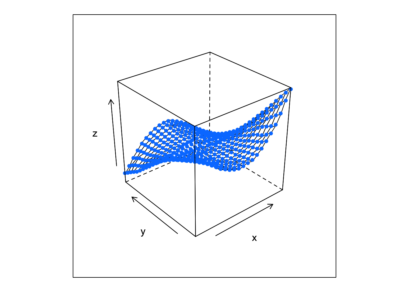

This looks like a dangerously good fit. It’s hard to see any difference between the data (the surface) and the fitted values (the points). Let’s see how the fitted values compare to the true function.

wireframe(true_z ~ x*y, data = df,
          panel = wire_cloud, point_z = df$fitted_z,
          pch = 16)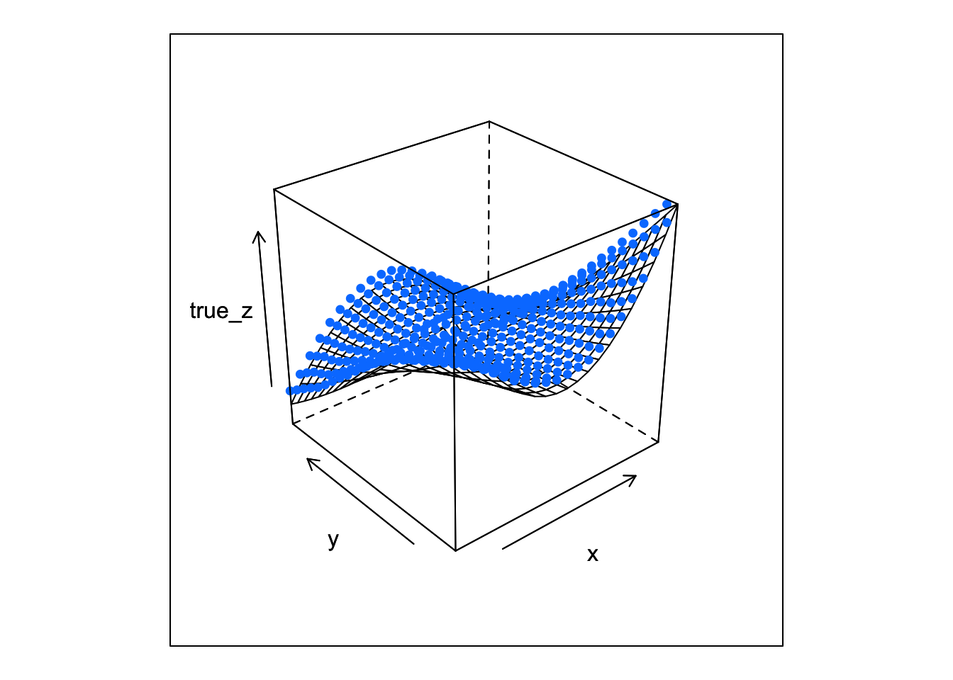

OK, now we can see the gaps.

For curiosity, we’ll take this one step further and see how the thin plate spline compares to a random forest. We won’t do anything fancy and just use the default values

library(randomForest)
fit_rf <- randomForest(z ~ x + y, df)
pred_rf <- predict(fit_rf)

df <- df %>% 
  mutate(fitted_rf = pred_rf)

wireframe(z ~ x*y, data = df,
          panel = wire_cloud, point_z = df$fitted_rf,
          pch = 16)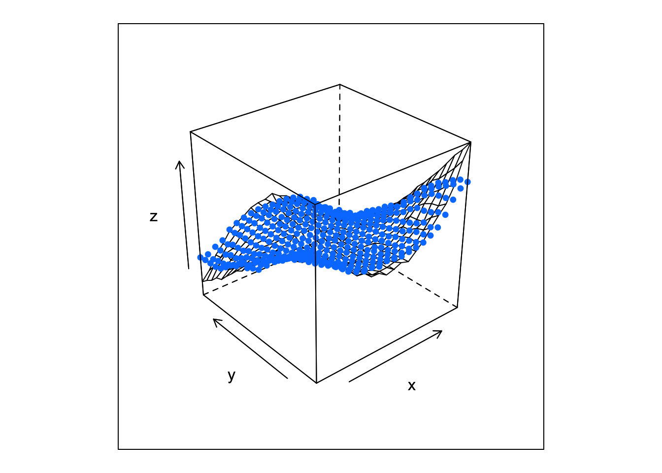

wireframe(true_z ~ x*y, data = df,
          panel = wire_cloud, point_z = df$fitted_rf,
          pch = 16)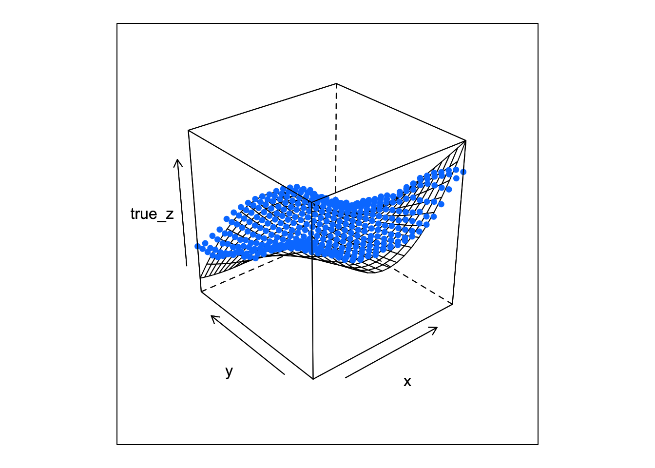

It’s pretty obvious from the plots that the thin plate spline is a better fit than the random forest. This probably has something to do with the fact that the true function is a polynomial and splines are polynomials at heart.

That’s it for thin plate splines. Next we will look at multivariate adaptive regression splines (MARS) and then finish of this section of nonlinear models with generalized additive models before moving on to nonlinear time series.