In a previous post I talked about how I am taking a self study course on nonlinear models. This is the first post on the topic with “real” content. The first topic I’ll be studying is splines. Here, I just want to provide an overview of splines. In future posts I will talk about different types of splines and provide some examples. Most of the material in this post is based on Chapter 7 of An Introduction to Statistical Learning and Chapter 5 of The Elements of Statistical Learning.
The Basic Idea
So what are splines? Essentially they are just piecewise polynomials with some smoothness conditions. We break the data into sections and fit polynomials to the data in each one of these sections.
The chunks are defined by knots. Knots can be any point but we usually use points in the data. For example, let’s say we have data that ranges from 1 to 10. Let’s also suppose we have data points at 2 and 6 and we use these as knots. These knots split our data into 3 chunks: points less than 2, points between 2 and 6, and points bigger than 6. We then fit polynomials to each one of these data chunks. This idea might be easier to see in a picture:
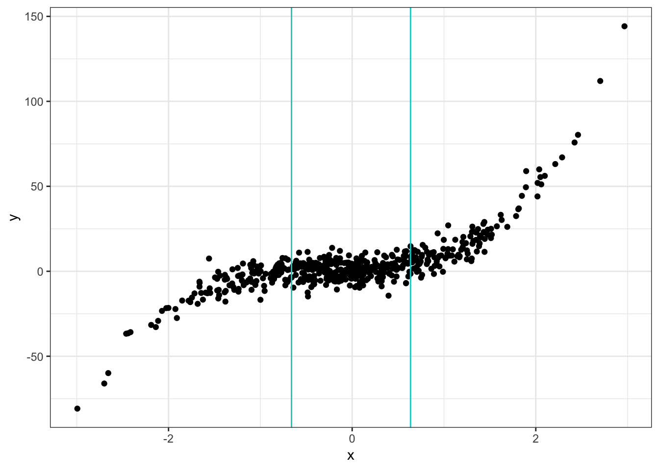
The vertical lines indicate where the knots are1.
To be splines though, we need some additional conditions. Instead of using any polynomial, we restrict our attention to polynomials that have continuous derivatives, up to a certain order, at each knot. So a spline is a polynomial of degree \(d\) that has continuous derivatives up to order \(d-1\) at each of the knots. That is, the first derivative is continuous, the second derivative is continuous, …, the \(d-1\)st derivative is continuous.
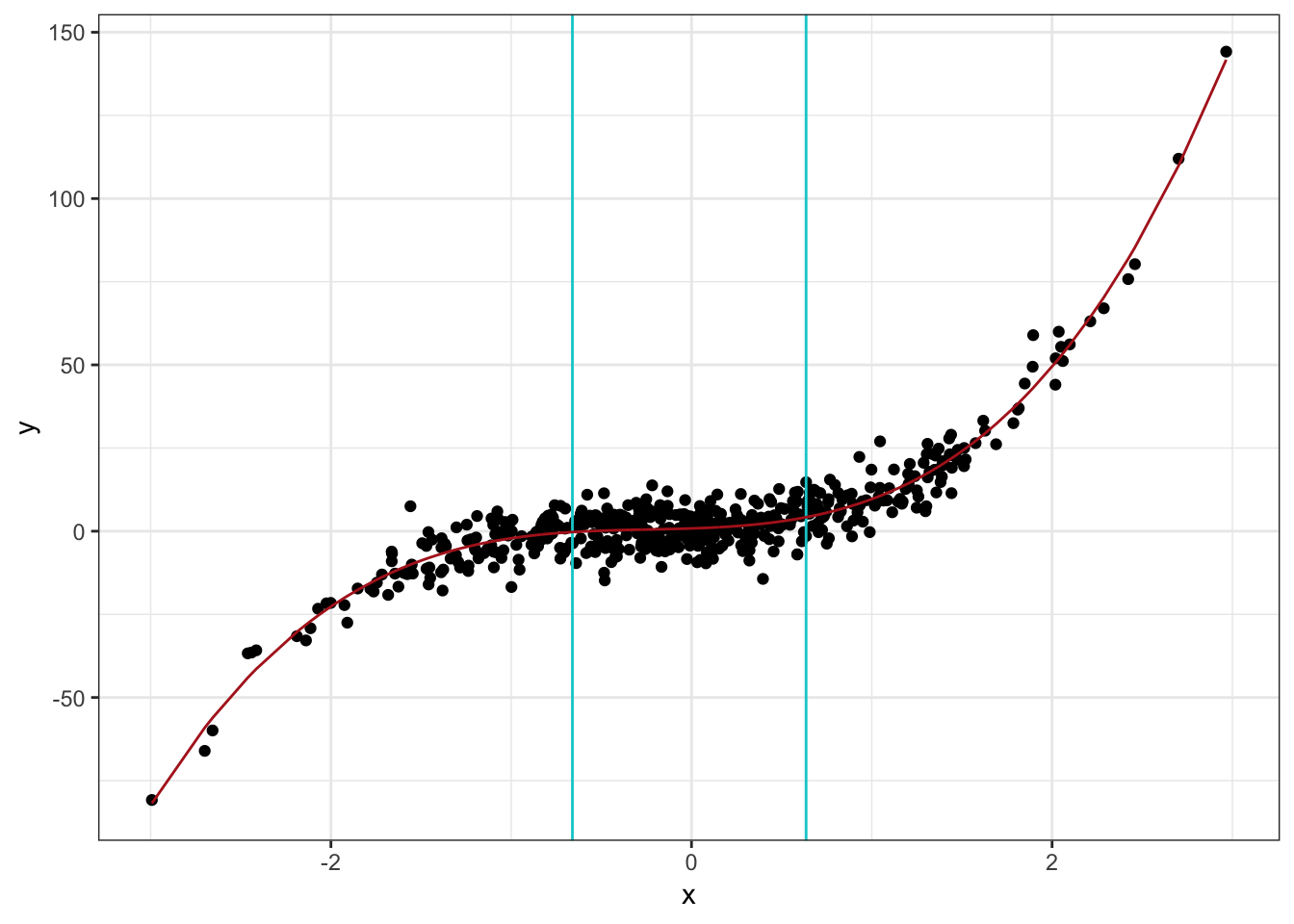
So in the plot above, we would fit one of these polynomials to the left chunk, the middle chunk, and the right chunk. The continuity restriction is to make sure the final fit is smooth. That it doesn’t have kinks2. A fitted spline model might look something like this:
“But wait” you say, “why don’t we just use polynomial terms in linear regression and forget about the whole spline business?” Well for one, splines can often perform better. They need a lower degree polynomial to achieve the same level of flexibility. A polynomial regression might need a high degree to achieve a good fit. Whereas with a spline, we can use lower degree polynomials with more knots. This makes splines more stable than polynomial regression. Gareth, et al. discuss this a bit more in Section 7.4.5 of An Introduction to Statistical Learning. Actually, polynomial regression and splines are part of a larger class of models that are based on the same underlying idea: basis functions.
Basis Functions
Basis functions generalize linear regression by allowing us to fit a linear model to nonlinear functions of the input data. We specify a set of basis functions, use them to transform the inputs, and then use these transformed variables as inputs to a linear model. The term basis in this context is just like the term basis from linear algebra. The set of functions we use define the basis of a vector space. In polynomial regression the basis functions are \(1, x, x^2, ..., x^d\). We could also use fancier functions like trigonometric polynomials (a la Fourier) or wavelets. But this post is about splines so let’s see what spline basis functions look like.
Some Math
Alright, now that we know the basic idea, let’s talk about some of the math behind splines. We’ll start by getting a feel for the basis function approach and then look at splines as a particular case. From this viewpoint, we are trying to estimate a model of the form \[ f(X) = \sum_{i=1}^k \beta_k h_k(X). \] Here, the \(\beta\)s are the coefficients and the \(h(X)\)s are the basis functions. In terms of the \(h(X)\)s, this is a linear model. Nonlinearity is introduced by choosing nonlinear functions for the \(h(X)\)s. Neural networks take the opposite approach. For neural networks we first take a linear combination of the coefficients and inputs and then we apply a nonlinear function to that. In the basis function approach we first apply nonlinear functions and then take a linear combination with the coefficients.
What kinds of functions can we use for the \(h(X)\)s? Hastie, et al. give a number of examples in The Elements of Statistical Learning that should feel very familiar. If we take \(h_k(X) = x_k\) for each \(x_k\), we are back to regular old linear regression. A common extension to this is \(h_k(X) = \log(x_j)\), taking the log transform of one or more input variables. Again, we could use fancy functions like Fourier terms but we will save that for later.
So what are the basis functions for splines? Let’s say we want to use cubic splines as these are the most common. As noted before, these are basically a cubic polynomial with additional conditions for continuity. The first part of a cubic spline basis is the regular polynomial basis: \(1, x, x^2, x^3\). Then we tack on a basis function of the form \[ h(x, \xi) = (x - \xi)_{+}^3 = \begin{cases} (x - \xi)^3 & \text{if } x > \xi \\ 0 & \text{if } x \le \xi. \end{cases} \] \(\xi\) stands for a knot. For each knot, we need to add one of these terms. The \(+\) means we only want to keep this term if \(x\) is larger than the knot \(\xi\). This takes care of the piecewise part, fitting a polynomial in a particular chunk of the data. Apparently, it also takes care of the continuity requirement. Let’s suppose were want to fit a cubic spline using two knots (as in the graphs we saw previously). Then the full set of basis functions would be \[ \begin{align*} h_1(X) &= 1 & h_2(X) &= X & h_3(X) &= X^2 \\ h_4(X) &= X^3 & h_5(X) &= (X - \xi_1)^3_{+} & h_6(X) &= (X - \xi_2)^3_{+}. \end{align*} \] If we wanted to use a degree \(d\) polynomial, then we would have \(1, X, ..., X^d\) along with \((X-\xi_1)^d_{+}\) and \((X-\xi_2)^d_{+}\). And if we wanted to include \(k\) knots we would also need to add \((X-\xi_i)^d_{+}\) for \(i = 3, 4, ..., k\).
Recap
Let’s summarize what we’ve seen so far. We talked about the basic idea behind splines: split the data into chunks and fit polynomials, with smoothness conditions, to each chunk. We can think of splines as extending polynomial regression which we often see in the context of linear regression. More generally, we can apply a set of (non)linear functions to the model inputs and then fit a linear model to the result. Lastly, we talked a bit about the math behind this idea and what the basis functions are for cubic splines with 2 knots and degree \(d\) splines with any number of knots.
If you find yourself wanting more spline goodness, don’t fret. We will be taking a deeper dive into splines in the coming weeks. And of course, we will get to see splines in action when we start fitting them to some data.